Download
1 / 39
450 likes | 774 Vues
Frontiers and Future of Multiphase Fluid Flow Modeling in Oil Reservoirs. Shuyu Sun Earth Science and Engineering program, Division of PSE, KAUST Applied Mathematics & Computational Science program, MCSE, KAUST Acknowledge: Mary F. Wheeler , The University of Texas at Austin

E N D
Frontiers and Future of Multiphase Fluid Flow Modeling in Oil Reservoirs • Shuyu Sun • Earth Science and Engineering program, Division of PSE, KAUST • Applied Mathematics & Computational Science program, MCSE, KAUST • Acknowledge: • Mary F. Wheeler, The University of Texas at Austin • Abbas Firoozabadi, Yale & RERI; Joachim Moortgat, RERI • Mohamed ElAmin, Chuanxiu Xu and Jisheng Kou, KAUST • Presented at 2010 CSIM meeting, KAUST Bldg. 2 (West), Level 5, Rm 5220, 11:10-11:35, May 1, 2010.
Single-Phase Flow In Porous Media
Single-Phase Flow in Porous Media • Continuity equation – from mass conservation: • Volumetric/phase behaviors – from thermodynamic modeling: • Constitutive equation – Darcy’s law:
Incompressible Single Phase Flow • Continuity equation • Darcy’s law • Boundary conditions:
DG scheme applied to flow equation • Bilinear form • Linear functional • Scheme: seek such that
Transport in Porous Media • Transport equation • Boundary conditions • Initial condition • Dispersion/diffusion tensor
DG scheme applied to transport equation • Bilinear form • Linear functional • Scheme: seek s.t. I.C. and
Example: Comparison of DG and FVM Upwind-FVM on 40 elements Linear DG on 20 elements Advection of an injected species from the left boundary under constant Darcy velocity. Plots show concentration profile at 0.5 PVI.
Example: Comparison of DG and FVM FVM Linear DG Advection of an injected species from the left. Plots show concentration profiles at 3 years (0.6 PVI).
Example: flow/transport in fractured media Locally refined mesh: FEM and FVM are better than FD for adaptive meshes and complex geometry
Adaptive DG example L2(L2) Error Estimators
A posteriori error estimate in the energy norm for all primal DGs Proof Sketch: Relation of DG and CG spaces through jump terms S. Sun and M. F. Wheeler, Journal of Scientific Computing, 22(1), 501-530, 2005.
Adaptive DG example (cont.) Anisotropic mesh adaptation
Adaptive DG example in 3D T=1.5 L2(L2) Error Estimators on 3D T=2.0 T=0.1 T=0.5 T=1.0
Two-Phase Flow In Porous Media
Two-Phase Flow Governing Equations • Mass Conservation • Darcy’s Law • Capillary Pressure • Saturation Summation Constraint
DG-MFEM IMPES Algorithm – Pressure Equ • If incompressible (otherwise treating it with a source term): • Total Velocity: • Pressure Equation: • MFEM Scheme: • Apply MFEM • Two unknown variables: Velocity Ua and Water potential
DG-MFEM IMPES Algorithm – Saturation Equ • Solve for the wetting (water) phase equation: • Relate water phase velocity with total velocity: • Saturation Equation (if using Forward Euler): • DG Scheme: • Apply DG (integrating by parts and using upwind on element interfaces) to the convection term.
Reservoir Description (cont.) • Relative permeabilities (assuming zero residual saturations): • Capillary pressure K=100md K=1md
Comparison: if ignore capillary pressure … With nonzero capPres With zero capPres Saturation at 10 years: Iter-DG-MFE
Saturation at 3 years Notice that Sw is continuous within each rock, but Sw is discontinuous across the two rocks Iter-DG-MFE Simulation
Saturation at 5 years Notice that Sw is continuous within each rock, but Sw is discontinuous across the two rocks Iter-DG-MFE Simulation
Saturation at 10 years Notice that Sw is continuous within each rock, but Sw is discontinuous across the two rocks Iter-DG-MFE Simulation
Multi-Phase Flow In Porous Media
Compositional Three-Phase Flow • Mass Conservation (without molecular diffusion) • Darcy’s Law
Example of CO2 injection • Initial Conditions: C10+H2O(Sw=Swc=0.1), 100 bar,160 F. • Inject water (0.1 PV/year) to 2 PV, then inject CO2 to 8 PV. Poutlet= 100 bar • Relative permeabilities: • Quadratic forms except nw=3. • Residual/critical saturations: • Sor = 0.40; Swc= 0.10; Sgc = 0.02 • Sgmax = 0.8; Somin = 0.2 • ; ; ;
Example (cont.) MFE-dG 0.1 PVI. MFE-dG 0.5 PVI. MFE-dG 0.2 PVI.
Example 3 (cont.) nC10 at 10% PVI CO2 nC10 at 200% PVI CO2
Remarks for Multiphase Flow • Framework has been established for advancing dG-MFE scheme for three-phase compositional modeling. In our formulation we adopt the total volume flux approach for the MFE. • dG has small numerical diffusion • CO2 injection • Swelling effect and vaporization • Reduction of viscosity in oil phase • Recovery by CO2 injection > Recovery by C1 > Recovery by N2
Modeling of Phase Behaviors for Reservoir Fluid
EOS Modeling of Phase Behaviors • PVT modeling: EOS • Peng-Robinson EOS • Cubic-plus-association EOS • Thermodynamic theory • Stability calculation • Tangent Phase Distance (TPD) analysis • Gibbs Free Energy Surface analysis • Flash calculation • Bisection method (Rachford-Rice equation) • Successive Substitution • Newton’s method
Three Monte Carlo movements in simulation • Particle displacements • Volume Change • Particle Transfer
Microstructure from the ab initio calculation The microstructure of the molecular models form the ab initio calculation The nearest neighbor interaction between the Water and Ethane T-shaped pair of water molecules
Water-ethane high pressure equilibria at T=523 K Experimental data are from Chemie-Ing. Techn. (1967), 39, 816 EoS: Statistical-Associating-Fluid-Theory (SAFT)