Injection oscillations in the PS
360 likes | 500 Vues
Injection oscillations in the PS. A. Huschauer, S. Gilardoni, C. Hernalsteens Acknowledgements: H. Bartosik, H. Damerau, K. Li, E. Métral , N. Mounet, G. Rumolo, G. Sterbini, R. Wasef, PS/PSB operations team HSC meeting , April 02, 2014. Overview. Motivation

Injection oscillations in the PS
E N D
Presentation Transcript
Injection oscillations in the PS A. Huschauer, S. Gilardoni, C. Hernalsteens Acknowledgements: H. Bartosik, H. Damerau, K. Li, E. Métral, N. Mounet, G. Rumolo, G. Sterbini, R. Wasef, PS/PSB operations team HSC meeting , April 02, 2014
Overview • Motivation • Measurements at injection and data analysis • HEADTAIL simulations • Analytic computations • Conclusions • Outlook
Motivation • slow losses observed for a few 100 μs after injection • losses in the injection region constitute one of the limitations for high intensity beams access very difficult in case of septum breakdown aperture and beam envelope in the injection region
Motivation • transverse oscillations observed at injection contribute to these losses emphasis on vertical oscillations. • oscillations currently cured with the TFB • however: underlying mechanism? • effect on future high intensity beams? • effect on future beams for the HL-LHC?
Measurements at injection • measurements done with the operational settings (mid - December 2012) • WBPU 94 used to observe transverse and longitudinal signals • fast build up of intra-bunch oscillations (few turns after injection) • oscillations primarily observed in the vertical plane • visible on different types of beams and each time the beam is injected more pronounced for high-intensity users Ip= 700 ∙1010 ppb Ip= 375 ∙1010 ppb TOF CNGS
Measurements at injection • different behavior of the oscillations depending on the PSB ring • example: CNGS, Ip= 750 ∙1010per PSB ring, 2 rings injected • optimized steering in the BTP-line reduces these oscillations
Data analysis First assumption: observations correspond to head-tail instability LHC TOF G. Sterbini • however: • time scale very short compared to one synchrotron period (~ 400 turns) • no mode structure appearing
Data analysis Increasing intra-bunch oscillation frequency (in the vertical plane) frequency spectrum based on a turn-by-turn FFT limited resolution due to small number of data points
Data analysis Detuning along the bunch noise of the baseline • sinusoidal fit computed over a window of 5 turns for each bin • repeated for the first 20 turns average value • assumption: linear machine, longitudinal motion negligible • programmed: Qv=6.33 • parabolic detuning observed (proportional to the line density)
HEADTAIL simulations • ImpedanceWake2D is used to obtain wall impedance and wake functions for a circular chamber • for the case of the PS the wake computations are based on a continuous stainless steel chamber with the shown dimensions (about 70% of the PS is equipped with this type)
Wake functions • wake functions for an elliptic geometry obtained from the circular one using the appropriate Yokoya factors
Longitudinal distribution measurement at PSB extraction distribution created by HEADTAIL
Discrimination between resistive and indirect space charge impedance currently considered slice Slicing of the bunch • ± 3 (HT input parameter) σz considered as total bunch length • bunch divided into 1700 equally thick slices Indirect space charge impedance decrease of the resistivity of the beam pipe allows determination of indirect space charge impedance only (10-7 10-14 in this case) effect of these slices on the current one accounts for resistive wall impedance only indirect space charge impedance is taken into account by using the SC wake function on the left and considering all slices
Discrimination between resistive and indirect space charge impedance resistive wall impedance only indirect space charge impedance only decoherence due to chromaticity very similar results as observed in the machine Indirect space charge effects are driving the observed phenomenon
Simulation results measurement simulation
Simulation results • indirect space charge impedance causes a real tune shift • no unstable behaviorof the beam observed • centroid motion decays because of natural chromaticity
Simulation results measurement simulation max. tune shift in this simulation is approx. 0.01 larger than in the measurement effect very sensitive to the longitudinal distribution
Different injection errors • without injection error no oscillations are observed • amplitude of the oscillation changes depending on the error • frequency remains the same
Effect of chromaticity ξv = -1.1 ξv = 0 ξv= -3
Intensity scan • intra-bunch oscillation frequency depends on intensity • simulations show a linear relationship between intensity and tune shift • recent simulations show that these oscillations will also be present on beams for the HL-LHC
Analytic computations 1) Determination of the coherent tune shift using Laslett’s formalism • choice of correct formula depends on whether magnetic fields penetrate the vacuum chamber • magnetic fields arising from bunching are always considered to be non-penetrating • but also transverse movement of the beam causes magnetic fields • these fields are considered non-penetrating if the skin depth satisfies ρ . . . resistivity of the beam pipe f0 . . . revolution frequency q . . . fractional tune μ . . . magnetic permeability d . . . thickness of the wall h . . . half height of the chamber
Analytic computations • in the case of the PS this relation holds true as • the appropriate formula for the tune shift then reads ac magnetic image from bunching magnetic image in poles ac magnetic image from betatron motion electric image B . . . bunching factor ξ1y, ε1y . . . vertical coh. and incoh. electric image coefficients ε2y. . . vertical incoherent dc magnetic image coefficient . . . fraction of the machine occupied by magnets g . . . distance vacuum chamber magnet pole magnetic images in the vacuum chamber
Analytic computations • the magnet poles are not taken into account in the simulations • the formula can then be rewritten as • however, this approach allows only to compute the maximum tune shift
Analytic computations • to compute a local tune shift one introduces the local bunching factor • B(s) depends on the longitudinal distribution Gaussian parabolic
Analytic computations • the resulting local tune shift reads • and the computation yields
Analytic computations Differences between Laslett’s formalism and tune shift obtained from simulations: • computed tune shift almost a factor 2 smaller than the one obtained by simulations • constant offset due to the term, which is not proportional to the bunching factor • reason for this: different regime of application, underlying assumptions, … ??
Analytic computations 2) Determination of the coherent tune shift using Sacherer’sformalism 2a) each slice is considered as uniform beam • which depends on the effective transverse impedance • hl(ω) is the beam spectrum for a uniform distribution N(s) . . . intensity of the slice R . . . machine radius R . . . half the length of a slice
Analytic computations • for very large values of the tune shift agrees with the simulations • corresponds to very few slices for a bunch with length of approx. 50 m
Analytic computations 2b) Gaussian bunch • for σz = 6.8 m one obtains ΔQmax= -0.056 • analysis of the first 20 turns of one simulation with a Gaussian bunch shows again a difference of approx. a factor 2 . . . RMS bunch length
Analytic computations Comparison with an FFT of the centroid motion over 100 turns • peak of the FFT (around 0.24) in agreement with tune obtained over the first 20 turns
Analytic computations – open questions • Where does the difference using the Laslett formalism come from? • Uniform beam: can we believe the convergence and the obtained tune shift? • For the shown case of a Gaussian bunch the FFT of the centroid motion and the analysis of the first 20 turns reveal similar information, why is the computation of the tune shift different?
Conclusion • The observed injection oscillations on the TOF beam can be explained by the effect of the indirect space charge impedance on a beam injected off-center. • No exponential growth of the centroid motion is observed – the purely imaginary impedance does not cause an instability. • The impedance of a simple elliptic geometry is sufficient to reproduce the measurements. • The oscillation frequency depends crucially on the longitudinal distribution. • The amplitude of the injection error only influences the amplitude of the oscillation and not its frequency. • Several open issues concerning the analytical model.
Outlook Publication to PRST-AB to be submitted this week (describing measurements and simulations) Additional means to reduce these oscillations: flat bunches ? After LS1: additional measurements on CNGS required to compare with simulations Further investigation of the different injection errors for bunches arriving from different rings and their effect on the observed oscillations Additional measurements at different energies.
Longitudinal distributions CNGS TOF
Vertical dipolar impedance wall impedance indirect space charge impedance “only”