Download
1 / 43
460 likes | 782 Vues
INTELLIGENT POWERTRAIN DESIGN. The BOND GRAPH Methodology for Modeling of Continuous Dynamic Systems and its Application in Powertrain Design. Jimmy C. Mathews Advisors: Dr. Joseph Picone Dr. David Gao. Outline. Dynamic Systems and Modeling Bond Graph Modeling Concepts

E N D
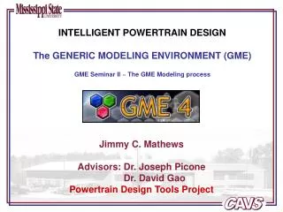
INTELLIGENT POWERTRAIN DESIGN The BOND GRAPH Methodology for Modeling of Continuous Dynamic Systems and its Application in Powertrain Design Jimmy C. Mathews Advisors: Dr. Joseph Picone Dr. David Gao
Outline • Dynamic Systems and Modeling • Bond Graph Modeling Concepts • Introduction and basic elements of bond graphs • Causality and state space equations • System Models and Applications using the Bond Graph Approach • Electrical Systems • Mechanical Systems • The Generic Modeling Environment (GME) and Bond Graph Modeling • Some Future Concepts
Dynamic Systems and Modeling • Dynamic Systems Related sets of processes and reservoirs (forms in which matter or energy exists) through which material or energy flows, characterized by continual change. • Common Dynamic Systems electrical, mechanical, hydraulic, thermal among numerous others. • Real-time Examples moving automobiles, miniature electric circuits, satellite positioning systems • Physical systems Interact, store energy, transport or dissipate energy among subsystems • Ideal Physical Model (IPM) The starting point of modeling a physical system is mostly the IPM. • To perform simulations, the IPM must first be transformed into mathematical descriptions, either using Block diagrams or Equation descriptions • Downsides – laborious procedure, complete derivation of the mathematical description has to be repeated in case of any modification to the IPM [3].
Computer Aided Modeling and Design of Dynamic Systems • Basic Concepts STEP 1: Develop an ‘engineering model’ STEP 2: Write differential equations STEP 3: Determine a solution STEP 4: Write a program Physical System Schematic Model The Big Question?? Classical Methods, Block Diagrams OR Bond Graphs GME + Matlab/Simulink Output Data Tables & Graphs Differential Equations Simulation and Analysis Software Fig 1. Modeling Dynamic Systems [1]
Fig 2. Subsystems of a bond graph [3] • Bond Graph Methodology • Invented by Henry Paynter in 1961, later elaborated by his students Dean C. Karnopp and Ronald C. Rosenberg • An abstract representation of a system where a collection of components interact with each other through energy ports and are placed in a system where energy is exchanged [2] • A domain-independent graphical description of dynamic behavior of physical systems • Consists of subsystems which can either describe idealized elementary processes or non-idealized processes [3] • System models will be constructed using a uniform notations for all types of physical system based on energy flow • Powerful tool for modeling engineering systems, especially when different physical domains are involved • A form of object-oriented physical system modeling
The Bond Graph Modeling Formalism • Bond Graphs • Conserves the physical structural information as well as the nature of sub-systems which are often lost in a block diagram. • When the IPM is changed, only the corresponding parts of a bond graphs have to be changed. Amenable to modification for ‘model development’ and ‘what if?’ situations. • Use analogous power and energy variables in all domains, but allow the special features of the separate fields to be represented. • The only physical variables required to represent all energetic systems are power variables [effort (e) & flow (f)] and energy variables [momentum p (t) and displacement q (t)]. • Dynamics of physical systems are derived by the application of instant-by-instant energy conservation. Actual inputs are exposed. • Linear and non-linear elements are represented with the same symbols; non-linear kinematics equations can also be shown. • Provision for active bonds. Physical information involving information transfer, accompanied by negligible amounts of energy transfer are modeled as active bonds.
Mechanical Rotation Hydraulic/Pneumatic Mechanical Translation Thermal Chemical/Process Engineering Electrical Magnetic • The Bond Graph Modeling Formalism (contd..) • A Bond Graph’s Reach Figure 3. Multi-Energy Systems Modeling using Bond Graphs
Fig 4. A series RLC circuit [4] Fig. 5Electric elements with power ports [4] • The Bond Graph Modeling Formalism (contd..) • Introductory Examples • Electrical Domain • Power Variables: • Electrical Voltage (u) & Electrical Current (i) • Power in the system: P = u * i • Constitutive Laws: uR = i * R • uC = 1/C * (∫i dt) • uL = L * (di/dt); or i = 1/L * (∫uL dt) Represent different elements with visible ports (figure 5) To these ports, connect power bonds denoting energy exchange The voltage over the elements are different The current through the elements is the same
The Bond Graph Modeling Formalism (contd..) • The R – L - C circuit • The common current becomes a “1-junction” in the bond graphs. • Note: the current through all connected bonds is the same, the voltages sum to zero 1 Fig 6. The RLC Circuit and its equivalent Bond Graph [4]
The Bond Graph Modeling Formalism (contd..) • Mechanical Domain • Mechanical elements like Force, Spring, Mass, Damper are similarly dealt with. • Power variables: Force (F) & Linear Velocity (v) • Power in the system: P = F * v • Constitutive laws: Fd = α * v Fs = KS * (∫v dt) = 1/CS * (∫ v dt) • Fm = m * (dv/dt); or v = 1/m * (∫Fm dt); Also, Fa = force Fig 7. The Spring Mass Damper System and its equivalent Bond Graph [4] • The common velocity becomes a “1-junction” in the bond graphs. Note: the velocity of all connected bonds is the same, the forces sum to zero)
The Bond Graph Modeling Formalism (contd..) • Analogies! • Lets compare! We see the following analogies between the mechanical and electrical elements: • The Damper is analogous to the Resistor. • The Spring is analogous to the Capacitor, the mechanical compliance corresponds with the electrical capacity. • The Mass is analogous to the Inductor. • The Force source is analogous to the Voltage source. • The common Velocity is analogous to the loop Current. • Notice that the bond graphs of both the RLC circuit and the Spring-mass-damper system are identical. Still wondering how?? • The bond graph modeling language is domain-independent. • Each of the various physical domains is characterized by a particular conserved quantity. Table 1 illustrates these domains with corresponding flow (f), effort (e), generalized displacement (q), and generalized momentum (p). • Note that power = effort x flow in each case.
The Bond Graph Modeling Formalism (contd..) • Table 1. Domains with corresponding flow, effort, generalized displacement and generalized momentum
e f B A • The Bond Graph Modeling Formalism (contd..) • Foundations of Bond Graphs • Based on the assumptions that satisfy basic principles of physics; a. Law of Energy Conservation is applicable b. Positive Entropy production c. Power Continuity • Closer look at Bonds and Ports • Power port or port: The contact point of a sub model where an ideal connection will be connected; location in a system where energy transfer occurs • Power bond or bond: The connection between two sub models; drawn by a single line (Fig. 8) • Bond denotes ideal energy flow between two sub models; the energy entering the bond on one side immediately leaves the bond at the other side (power continuity). (directed bond from A to B) Energy flow along the bond has the physical dimension of power, being the product of two variables effort and flow called power-conjugated variables Power bond viewed as interaction of energy and bilateral signal flow Fig. 8 Energy flow between two sub models represented by ports and bonds [4]
The Bond Graph Modeling Formalism (contd..) • Bond Graph Elements – 9 elements • Drawn as letter combinations (mnemonic codes) indicating the type of element. • C storage element for a q-type variable, e.g. capacitor (stores charge), spring (stores displacement) • L storage element for a p-type variable, e.g. inductor (stores flux linkage), mass (stores momentum) • R resistor dissipating free energy, e.g. electric resistor, mechanical friction • Se, Sf sources, e.g. electric mains (voltage source), gravity (force source), pump (flow source) • TF transformer, e.g. an electric transformer, toothed wheels, lever • GY gyrator, e.g. electromotor, centrifugal pump • 0, 1 0 and 1 junctions, for ideal connection of two or more sub-models
Fig. 9 Examples of C - elements [4] • The Bond Graph Modeling Formalism (contd..) • Storage Elements • Two types; C – elements & I – elements; q–type and p–type variables are conserved quantities and are the result of an accumulation (or integration) process; they are the state variables of the system. • C – element (capacitor, spring, etc.) • q is the conserved quantity, stored by accumulating the net flow, f to the storage element • Resulting balance equation dq/dt = f An element relates effort to the generalized displacement 1-port element that stores and gives up energy without loss
Fig. 10 Examples of I - elements [4] • The Bond Graph Modeling Formalism (contd..) I – element (inductor, mass, etc.) p is the conserved quantity, stored by accumulating the net effort, e to the storage element. Resulting balance equation dp/dt = e For an inductor, L [H] is the inductance and for a mass, m [kg] is the mass. For all other domains, an I – element can be defined.
The Bond Graph Modeling Formalism (contd..) R – element (electric resistors, dampers, frictions, etc.) R – elements dissipate free energy and energy flow towards the resistor is always positive. Algebraic relation between effort and flow, lies principally in 1st or 3rd quadrant. e = r * (f) Fig. 11 Examples of Resistors [4] If the resistance value can be controlled by an external signal, the resistor is a modulated resistor, with mnemonic MR. E.g. hydraulic tap
The Bond Graph Modeling Formalism (contd..) Sources (voltage sources, current sources, external forces, ideal motors, etc.) Sources represent the system-interaction with its environment. Depending on the type of the imposed variable, these elements are drawn as Se or Sf. Fig. 12 Examples of Sources [4] When a system part needs to be excited by a known signal form, the source can be modeled by a modulated source driven by some signal form (figure 13). Fig. 13 Example of Modulated Voltage Source [4]
The Bond Graph Modeling Formalism (contd..) Transformers (toothed wheel, electric transformer, etc.) An ideal transformer is represented by TF and is power continuous (i.e. no power is stored or dissipated). The transformations can be within the same domain (toothed wheel, lever) or between different domains (electromotor, winch). e1 = n * e2 & f2 = n * f1 Efforts are transduced to efforts and flows to flows; n is the transformer ratio. Fig. 14 Examples of Transformers [4]
The Bond Graph Modeling Formalism (contd..) Gyrators (electromotor, pump, turbine) An ideal gyrator is represented by GY and is power continuous (i.e. no power is stored or dissipated). Real-life realizations of gyrators are mostly transducers representing a domain-transformation. e1 = r * f2 & e2 = r * f1 r is the gyrator ratio and is the only parameter required to describe both equations. Fig. 15 Examples of Gyrators [4]
The Bond Graph Modeling Formalism (contd..) Junctions Junctions couple two or more elements in a power continuous way; there is no storage or dissipation at a junction. 0 – junction Represents a node at which all efforts of the connecting bonds are equal. E.g. a parallel connection in an electrical circuit. The sum of flows of the connecting bonds is zero, considering the sign. 0 – junction can be interpreted as the generalized Kirchoff’s Current Law. Equality of efforts (like electrical voltage) at a parallel connection. Fig. 16 Example of a 0-Junction [4]
The Bond Graph Modeling Formalism (contd..) 1 – junction Is the dual form of the 0-junction (roles of effort and flow are exchanged). Represents a node at which all flows of the connecting bonds are equal. E.g. a series connection in an electrical circuit. The efforts of the connecting bonds sum to zero. 1- junction can be interpreted as the generalized Kirchoff’s Voltage Law. In the mechanical domain, 1-junction represents a force-balance, and is a generalization of Newton’ third law. Additionally, equality of flows (like electrical current) through a series connection. Fig. 17 Example of a 1-Junction [4]
The Bond Graph Modeling Formalism (contd..) Some Miscellaneous Stuff! Power Direction: The power is positive in the direction of the power bond. If power is negative, it flows in the opposite direction of the half-arrow. Typical Power flow directions R, C, and I elements have an incoming bond (half arrow towards the element) Se, Sf: outgoing bond TF– and GY–elements (transformers and gyrators): one bond incoming and one bond outgoing, to show the ‘natural’ flow of energy. These are constraintson the model!
Fig. 18 Causality Assignment [4] • The Bond Graph Modeling Formalism (contd..) • Causal Analysis • Causal analysis is the determination of the signal direction of the bonds • Establishes the cause and effect relationships between the bonds • Indicated in the bond graph by a causal stroke; the causal stroke indicates the direction of the effort signal. • The result is a causal bond graph, which can be seen as a compact block diagram. • Causal analysis covered by modeling and simulation software packages that support bond graphs; Enport, MS1, CAMP-G, 20 SIM
e e f Se Se f e f Sf e2 e1 TF e2 e1 TF n f1 f2 f1 f2 n e2 e2 e1 e1 e TF f1 f2 TF Sf n n f1 f2 f • The Bond Graph Modeling Formalism (contd..) Causal Constraints: Four different types of constraints need to be discussed prior to following a systematic procedure for bond graph formation and causal analysis
e2 e2 e1 e1 GY GY f1 f1 f2 f2 r r 0 1 C L C L • The Bond Graph Modeling Formalism (contd..) OR any other combination where exactly one bond brings in the effort variable OR any other combination where exactly one bond has the causal stroke away from the junction
R R • The Bond Graph Modeling Formalism (contd..) Some notes on Preferred Causality (C, I) Causality determines whether an integration or differentiation w.r.t time is adopted in storage elements. Integration has a preference over differentiation because: 1. At integrating form, initial condition must be specified. 2. Integration w.r.t. time can be realized physically; Numerical differentiation is not physically realizable, since information at future time points is needed. 3. Another drawback of differentiation: When the input contains a step function, the output will then become infinite. Therefore, integrating causality is the preferred causality. C-element will have effort-out causality and I-element will have flow-out causality
+ - 0:U23 0:U12 U0 U2 U3 U1 • Examples • Electrical Circuit # 1 (R-L-C) and its Bond Graph model U2 U3 U1 • 0 0 0 • 0 1 0 1 0
R : R I : L 0:U23 0:U12 C : C 1 0 1 0 0 Se : U U3 U2 U1 R : R 1 I : L Se : U C : C • Examples (contd..)
R : R R : R R : R 1 1 1 I : L I : L I : L Se : U Se : U Se : U C : C C : C C : C • Examples (contd..) • The Causality Assignment Algorithm: 1. 2. 3.
R1 C2 R2 L1 R3 C1 L1 C2 C1 R3 R1 R2 • Examples (contd..) • Electrical Circuit # 2 and its Bond Graph model • A DC Motor and its Bond Graph model
SE Transmission Ratio TF τL τL ωL ωL ωi 0 0 TF 1 τR τR ωR ωR Differential Ratio SF TF Drive Shaft Compliance C 1 ωi 0 TF • Examples (contd..) • A Drive Train Schematic and its Bond Graph model Bond Graph without Drive Shaft Compliance [9] A Drive Train Schematic [9] Bond Graph with Drive Shaft Compliance [9]
Examples (contd..) Schematic of a tire and suspension [9] Suspension model for one wheel and anti-roll bar Bond Graph of a wheel-tire system – Vertical Dynamics [9] Bond Graph of a wheel-tire system – Longitudinal Dynamics [9] Bond Graph of a wheel-tire system – Transverse Dynamics [9] • Schematic for Tire and Suspension and their Bond Graph model
2 1 4 3 R : R 1 I : L Se : U C : C • Generation of Equations from Bond Graphs • A causal bond graph contains all information to derive the set of state equations. • Either a set of Ordinary first-order Differential Equations (ODE) or a set of Differential and Algebraic Equations (DAE). • Write the set of mixed differential and algebraic equations. • For a bond graph with n bonds, 2n equations can be formed, n equations each to compute effort and flow or their derivatives. • Then, the algebraic equations are eliminated, to get final equations in state-variable form. Fig. 19 Bond Graph of a series RLC circuit • For the given RLC circuit, Se = e1= U; • e2 = R * f2; • (de3/dt) = (1/C) * f3; • (df4/dt) = (1/L) * e4; • f1 = f4; f2 = f4; f3 = f4; • e4 = e1 - e2 - e3 • Hence, e1 - e2 - e3 = U – (R * f2) – e3 = U – (R * f4) – e3 • (df4/dt) = (1/L) * (U – (R * f4) – e3) - - - - - - - (i)
Generation of Equations from Bond Graphs (contd..) • Also, (de3/dt) = (1/C) * f3 = (1/C) * f4 - - - - - - - - (ii) • In matrix form, (dx/dt) = Ax + Bu • (de3/dt) 0 1/C e3 0 • = + U • (df4/dt) -1/L -R/L f4 1/L
Applications in GME Metamodeling Environment • RLC Circuit
Applications in GME Metamodeling Environment (contd..) • DC Motor
Applications in GME Metamodeling Environment (contd..) DC Motor model
Future Concepts • Defining the GME Approach for analysis of Bond Graphs [1]
Bond Graph Interpreters in GME ?? Fig 20. The Simulation Generation Process [7] • Future Concepts (contd..) • Creating Bond Graph Interpreters
Future Concepts (contd..) • Advanced Bond Graph Techniques • Expansion of Bond Graphs to Block Diagrams • Bond Graph Modeling of Switching Devices • Hierarchical modeling using Bond Graphs • Use of port-based approach for Co-simulation
References • Granda J. J, “Computer Aided Design of Dynamic Systems” http://gaia.csus.edu/~grandajj/ • Wong Y. K., Rad A. B., “Bond Graph Simulations of Electrical Systems,” The Hong Kong Polytechnic University, 1998 • http://www.ce.utwente.nl/bnk/bondgraphs/bond.htm • Broenink J. F., "Introduction to Physical Systems Modeling with Bond Graphs,"University of Twente, Dept. EE, Netherlands. • Granda J. J., Reus J., "New developments in Bond Graph Modeling Software Tools: The Computer Aided Modeling Program CAMP-G and MATLAB," California StateUniversity, Sacramento • http://www.bondgraphs.com/about2.html • Vashishtha D., “Modeling And Simulation of Large Scale Real Time Embedded Systems,” M.S. Thesis, Vanderbilt University, May 2004 • Hogan N. "Bond Graph notation for Physical System models," IntegratedModeling of Physical System Dynamics • Karnopp D., “System Dynamics: Modeling and simulation of mechatronic systems”