Download
1 / 13
130 likes | 157 Vues
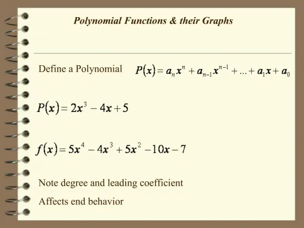
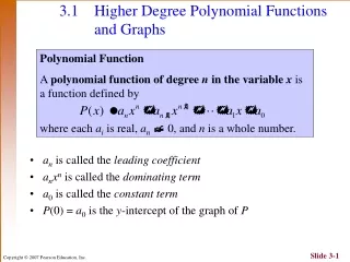
3.1 Higher Degree Polynomial Functions and Graphs. Polynomial Function A polynomial function of degree n in the variable x is a function defined by where each a i is real, a n 0, and n is a whole number. a n is called the leading coefficient

E N D
3.1 Higher Degree Polynomial Functions and Graphs Polynomial Function A polynomial function of degree n in the variable x is a function defined by where each ai is real, an 0, and n is a whole number. • an is called the leading coefficient • anxn is called the dominating term • a0 is called the constant term • P(0) = a0 is the y-intercept of the graph of P
3.1 Cubic Functions: Odd Degree Polynomials • The cubic function is a third degree polynomial of the form • In general, the graph of a cubic function will resemble one of the following shapes.
3.1 Quartic Functions: Even Degree Polynomials • The quartic function is a fourth degree polynomial of the form • In general, the graph of a quartic function will resemble one of the following shapes. The dashed portions indicate irregular, but smooth, behavior.
3.1 Extrema • Turning points – where the graph of a function changes from increasing to decreasing or vice versa • Local maximum point – highest point or “peak” in an interval • function values at these points are called local maxima • Local minimum point – lowest point or “valley” in an interval • function values at these points are called local minima • Extrema – plural of extremum, includes all local maxima and local minima
3.1 Number of Local Extrema • A linear function - degree 1 - no local extrema. • A quadratic function - degree 2 - one extreme point. • A cubic function - degree 3 - at most two local extrema. • A quartic function -degree 4 - at most three local extrema. • Extending this idea: Number of Turning Points The number of turning points of the graph of a polynomial function of degree n 1 is at most n – 1.
3.1 End Behavior Let axn be the dominating term of a polynomial function P. • n odd • If a positive, the graph of P falls on the left and rises on the right. • If a is negative, the graph of P rises on the left and falls on the right. • n even • If a > 0, the graph of P opens up. • If a < 0, the graph of P opens down.
3.1 Determining End Behavior Match each function with its graph. Solution: B. A. C. D. f matches C, g matches A, h matches B, k matches D.
3.1 Analyzing a Polynomial Function • Determine its domain. • Determine its range. • Use its graph to find approximations of local extrema. • Use its graph to find the approximate and/or exact x- intercepts. Solution • Since P is a polynomial, its domain is (–,). • Because it is of odd degree, its range is (–,).
3.1 Analyzing a Polynomial Function • Two extreme points that we approximate using a graphing calculator: local maximum point (– 2.02,10.01), and local minimum point (.41, – 4.24). Looking Ahead to Calculus The derivative gives the slope of f at any value in the domain. The slope at local extrema is 0 since the tangent line is horizontal.
3.1 Analyzing a Polynomial Function (d) We use calculator methods to find that the x-intercepts are –1 (exact), 1.14(approximate), and –2.52 (approximate).
3.1 Comprehensive Graphs • The most important features of the graph of a polynomial function are: • intercepts, • extrema, • end behavior. • A comprehensive graph of a polynomial function will exhibit the following features: • all x-intercepts (if any), • the y-intercept, • all extreme points (if any), • enough of the graph to exhibit end behavior.
3.1 Determining the Appropriate Graphing Window The window [–1.25,1.25] by [–400,50] is used in the following graph. Is this a comprehensive graph? Solution Since P is a sixth degree polynomial, it can have up to 6 x-intercepts. Try a window of [-8,8] by [-1000,600].