Download
1 / 28
280 likes | 308 Vues
This paper explores different recovery schemes for fault-tolerant systems in distributed computing environments. It covers single process, greedy, golomb, modulo, and trapezium recovery schemes, and discusses their optimality. The paper concludes with insights and findings on recovery schemes.

E N D
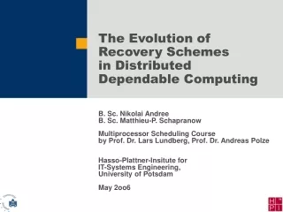
The Evolution of Recovery Schemes in Distributed Dependable Computing B. Sc. Nikolai AndreeB. Sc. Matthieu-P. Schapranow Multiprocessor Scheduling Courseby Prof. Dr. Lars Lundberg, Prof. Dr. Andreas Polze Hasso-Plattner-Insitute forIT-Systems Engineering,University of PotsdamMay 2oo6
Agenda • Problem Definition • Trivial Recovery Schemes • Definitions • Recovery Schemes • Single Process Recovery Schemes • Greedy Recovery Schemes • Golomb Recovery Schemes • Modulo Recovery Schemes • Trapezium Recovery Schemes • Conclusions
Problem Definition • Fault tolerance: • “Ability of a system to respond gracefully to an unexpected hardware/software failure” • Recovery List • List of computers to distribute the work, if the current computer breaks down, i.e. one list per processSm = <s1, s2, ..., sn-1> • Recovery Scheme • Totality of all recovery lists for processes in one cluster; • General recovery scheme • Every element in the recovery list must be distinct
Problem Definition (contd.) System 0 System 0 Process 1 R1: <0, 3, 2> System 1 Process 2 R2: <1, 0, 3> System 2 Process 3 R3: <0, 1, 2> System 3 Process 0R0: <1, 2, 3> Assumptions: one process per system initially and static recovery schemes Ri defines the recovery list for process i.
Problem Definition (contd.) System 0 Process 1 R1: <0, 3, 2> System 1 Process 2 R2: <1, 0, 3> System 2 System 3 System 3 Process 3R3: <0, 1, 2> Process 0R0: <1, 2, 3>
Problem Definition (contd.) System 0 Process 1 R1: <0, 3, 2> System 1 Process 2 R2: <1, 0, 3> System 2 System 3 System 3 Process 0R0: <1, 2, 3> Process 3R3: <0, 1, 2>
Trivial Recovery Schemes • Ri = { (r0 + i) mod n, (r1 + i) mod n, ..., (rn + i) mod n }, 0 i n. • For n = 4 computer systems: • R0: < 1, 2, 3 > • R1: < 2, 3, 0 > • R2: < 3, 0, 1 > • R3: < 0, 1, 2 > ...and all of its permutations R(n) = set of regular recovery schemes of length n trivial regularnon-optimalmodulo recovery scheme
Definitions • Load on the most heavily loaded computer system in the environment • L(n, x, {c0,…,cx-1}, RS) with n > x. • n – number of computers in the cluster • x – i.e. |{c0,…,cx-1} | the number of computers currently down in the cluster • {c0,…,cx-1} – set of computers currently down in the cluster • RS – defines the recovery scheme • L(4,2,{0,3},RS) = 3 (cf. slide 5) • L(4,2,{0,1},RS) = 2 • L(n, x, RS) = max L(n, x, {c0,…,cx-1}, RS) for all sets{c0,…,cx-1} • I.e. the worst-case scenario for the recovery scheme RS • L(4,2,RS) = 3 • Bound Vector BV • BV of the length l = (2{2}, 3{3}, 4{4}, …, k) with k{t} is equivalentto t-times the value k, i.e. B(x) = sqrt(2(x+1)) + ½ • E.g. BV of the length 6: (2, 2, 3, 3, 3, 4) • Increases at indices ½*l*(l+1), l 1, i.e. BV(½*l*(l+1)) = l+1
Definitions (contd.) • Relation smaller than of recovery schemes • V(L(n,RS)) := ( L(n,1,RS), …, L(n,n-1,RS) ) • Vector containing n-1 entries • I.e. the worst-case scenario for 1 to n-1 broken computers • V(L(n,RS1)) V(L(n,RS2)) if • L(n,y,RS1) < L(n,y,RS2) + y | 1 < y n AND L(n,z,RS1) = L(n,z,RS2) for z < y • I.e. compontent-wise comparison • E.g. Let V1 = V(L(4, RS1) = (2, 2, 4)AND V2 = V(L(4, RS2) = (2, 3, 4) V1 V2 • VL = min V(L(n,RS)) for all recovery schemes RS • I.e. a vector of the length n-1 • T1: n/(n-x) ≤ VL(x), i.e. the x-th entry in VL, e.g. VL(1) ≥ 4/(4-1) ≥ 2, VL(2) = 2, VL(3) ≥ 4 • T2: BV ≤ VL, e.g. BV = (2, 2, 3) • T1 T2 MV(x) := B(x) = max ( BV(x), n/(n-x) ), e.g. B(1) = 2, B(2) = 2, B(3) = 4
Definitions (contd.) • Regular Recovery Schemes • All recovery lists contains the same structure • All recovery lists are constructed using one recovery list (often: R0) • Optimality • x‘ = MV(x), i.e. the maximal number of processes on the same computer after x crashes equals MV(x) • In other words: V(L(n,RS)) = B = MV
ld n Recovery Schemes • Aka single-process recovery scheme [8] • x m | L(n,x, RSSP) = B(x), m = ld n • BV of length eleven: (2, 2, 3, 3, 3, 4, 4, 4, 4, 5, 5) • E.g. n = 15, m = 3, L( 15, 3, RSSP) = B(3) = 3 max. load n = 1000, m = 9, L(1000, 9, RSSP) = B(9) = 4 max. load • R0 = { ( 21-1), (22-1), …, (2m-1), (2m-2m-2-1), (2m-2m-3-1), (2m-3*2m-3-1), (2m-5*2m-3-1), (2m-2m-4-1), (2m-3*2m-4-1), (2m-5*2m-4-1), (2m-7*2m-4 -1), (2m-9*2m-4 -1),(2m-11*2m-4-1), (2m-13*2m-4-1),(2m-2m-5-1), (2m-3*2m-5-1), …, (i+2m-29*2m-5 -1), …, (2m-2m-x-1), (2m-3*2m-x-1), …, (2m-(2x-3)*2m-x-1), … (2m-20 -1), (2m-3*20 -1), …, (2m-(2m-3)*20 -1)} • If n is not a power of two m = ld n and remove all entries n in R0 • E.g.: R0 = { 1, 3, 7, 11, (15), 13, 9, 5, 14, 12, 10, 8, 6, 4, 2} Guarantees optimal evenly redistribution of work only up to nine broken systems in a cluster of 1000 systems!
Greedy Recovery Schemes • Aka improved recovery scheme [3] • Optimal for x max(i) crashed systems, so that R0(i) < n • Step vector r(x) = min(j N) • R0(x) • (1 a1 b1 x) AND • (1 a2 b2 x) AND • ((a1 a2) OR (b1 b2)) • E.g., n = 97, R0 = ( 1, 3, 7, 12, 20, 30, 44, 65, 80, 96 ) first 10 entries using r(l). • reduced step vector r’(l) = ( 1, 2, 4, 5, 8, 10, 14, 21, 15, 16 )
Greedy Recovery Schemes (contd.) Excluding value one may improve the results for the given recovery list This indicates the all sums of the reduced step vector r’(l) for n = 97.Sj indicate the sum of the subsequence with the length j starting at position i.E.g. The sum of the subsequent with the length 5 starting at position 3 is S5(3) = 62.
Greedy Recovery Schemes (contd.) • E.g., for n = 1000 optimal behavior is guaranteed for x 26 broken systems. • Comparison: For n = 1000 Ld Recovery Scheme guarantees optimality for x 9 broken systems. Greedy Recovery Scheme guarantees optimality for almost three-times more broken systems than Ld Recovery Schemes!
Golomb Ruler Recovery Schemes • Golomb Ruler • A sequence of positive integers • No two distinct pairs of numbers of the set have the same difference • Numbers are called marks • Difference between any two marks is called distance • Optimal Golomb Ruler (OGR) is the shortest ruler for a given number of marks • NP-hard to calculate • Thus, only OGRs up to length 24 are proved in May 2006 OGR of the length 4: absolute distances: 0-1-4-9-11 (resp. as sequence of distances 1-3-5-2) can measure all length up to 11: Distances 1, 2, 3, 5 are given directly, 4 = 1 + 3, 7 = 2 + 5, 8 = 3 + 5, 9 = 1 + 3 + 5, 10 = 2 + 3 + 5, 11 = 1 + 2 + 3 + 5 are calculated.
Golomb Ruler Recovery Schemes (contd.) • Let Gn be the Golomb Ruler with sum n + 1 • gn = x describes number of crashed systems to guarantee optimality for • How to construct? • Find an optimal Golomb sequence n • If necessary fill up sequence with remaining computer systems. • E.g. G12 generates the list {1, 4, 9, 11, 2, 3, 5, 6, 7, 8, 10} • Longest OGR in May 2006 G24 = {0, 9, 33, 37, 38, 97, 122, 129, 140, 142, 152, 191, 205, 208, 252, 278, 286, 326, 332, 353, 368, 384, 403, 425} Guarantees optimal evenly redistribution of work up to 34 broken systems in a cluster of 1000 systems!
Golomb Ruler Recovery Schemes (contd.) • Application available at http://www.myhpi.de/~schapran/mps/ • Problems • How to determine the size of the number room • When to stop bruteforce to save time
Golomb Ruler Recovery Schemes (contd.) • Optimal Golomb Sequences vs. Greedy Sequences [4]
Modulo Recovery Schemes • Modulo-n sequence • Sequence of positive integers {an}, n 0 • For all n > ½ * l * (l+1), l is the length of the sequence • No distinct pairs {ae, af}, {ag, ah}, e > f, g > hhave the same difference modulo n • I.e. a special case of a Golomb Ruler with l marks d1, d2, d3, …, dl • all differences (dj – di) % n are distinct, i < j AND • all differences (dj – di) % n are non-zero • E.g. Modulo-11 sequence • n = 11 > 10, l = 4: {1, 6, 3, 10}, {2, 1, 6, 9}, {3, 7, 9, 8}, … • Modulo Recovery List MR0,n • MR0,11 = {1, 6, 3, 10, 2, 4, 5, 7, 8, 9} • MR0,11 = {2, 1, 6, 9, 3, 4, 5, 7, 8, 10} • MR0,11 = {3, 7, 9, 8, 1, 2, 4, 5, 6, 10} • Underlined is the modulo-12 sequence of the length l=4 • MRi,n = {(i+MR0,n(1) % n), (i+MR0,n(2) % n), …, (i+MR0,n(1) % (n-1))}
Modulo Recovery Schemes (contd.) • Optimality • Optimality is guaranteed for x = max(i) with MR0,n(i) < n • I.e. the set of numbers constructed via distinct pairs • Perfect Modulo Ruler • Modulo sequence with exact distinct differences • Only possible for l 5. • Modulo Recovery Scheme vs. Golomb Recovery Scheme • E.g. n = [92, 106] • MR0,100: {1, 6, 78, 47, 20, 24, 45, 74, 57, 17, 8, 87, 2, 3, 4, 5, 7, 9, 10, 11, 12, …} • OGR0,100: {2, 6, 24, 29, 40, 43, 55, 68, 75, 76, 85, 1, 3, 4, 5, 7, 8, 9, 10, 11, …} Modulo sequences only known for max. 92 systems per cluster, OGRs known up to 426 systems (24 marks), proving on 480 systems (25 marks) [9].
Modulo Recovery Schemes (contd.) • Modulo Recovery Scheme vs. Golomb Recovery Scheme [5]
Trapezium Recovery Schemes • Finding a proper sequence S = < s1, s2, …, sn-1 > • Sum of all elements up to k in the sequence S is max. n • l = ½ * (sqrt(8k +9) -1) , with k crashed nodes • First l crash routes are disjoint, i.e. #nodes = ½ * l * (l+1) • Following ½ * l * (l+1) -l crash routes contain at least l unique values • Let Ci be a crash route, i.e. < s1+s2+…+si, s2+…+si, si >, thus crash routes are read diagonally, i.e. C1 = {1}, C2 = {4, 3}, etc.
Trapezium Recovery Schemes (contd.) • Increasing load • Each time the unique part of a crash route is passed • Load on Z increases, if Z – C1 = Z – C1(1) if Z – C2 = Z – C2(1) AND Z – C2(2) if Z – C3 = Z – C3(1) AND Z – C3(2) AND Z – C3(3), etc. • E.g. Load on Z increases, if Z – 1 crashes if Z – 4 AND Z – 3 if Z – 6 AND Z – 5 AND Z – 2
Trapezium Recovery Schemes (contd.) • Optimality • E.g. n = 100, Trapezium RS guarantees optimality up to 15 broken systems • Golomb RS guarantees optimality up to 11 broken systems • n = 1000, Trapezium RS guarantees optimality up to 78 broken systems • Golomb RS guarantees optimality up to 34 broken systems For n = 100, Trapezium RS improves performance approx. 4/3-times. For n = 1000, Trapezium RS improves performance even 7/3-times!
Conclusions … Short Calculation Time Perfomance of Recovery Scheme Trapezium Modulo Golomb Greedy Ld Trivial
Conclusions (contd.) • Two major types of algorithm for recovery list creation can be distinguished • Distinct pair search • Modulo • Comparing the given algorithms show the following performance relation:Ld < Greedy < Golomb < Modulo < Trapezium • Improvements • Reformulation of a given mathematical problem • Involving known statistical results results in performance improvements • Open improvents, what to expect…
References • [1] Analysis of the Golomb Ruler and the Sidon Set Problems, and Determination of Large, Near-Optimal Golomb Rulers, Apostolos Dimitromanolakis, Department of Electronic and Computer Engineering, Technical University of Crete, June 2002 • [2] Optimal Recovery Schemes in Fault Tolerant Clusters and Distributed Computing, Lars Lundberg, Department of Software Engineering and Computer Science Blekinge Institut of Technology, Sweden, March 2005 • [3] Recovery Schemes for High Availability and High Performance Distributed Real-Time Computing, Lars Lundberg et al, Department of Software Engineering and Computer Science, Blekinge Institute of Technology, S-372 25 Ronneby, Sweden, 2003 • [4] Using Golomb Rulers for Optimal Recovery Schemes in Fault Tolerant Distributed Computing, Kamilla Klonowska, Lars Lundberg, Håkan Lennerstad, Department of Software Engineering and Computer Science, Blekinge Institute of Technology, S-372 25 Ronneby, Sweden, 2003 • [5] Using Modulo Rulers for Optimal Recovery Schemes in Distributed Computing, Kamilla Klonowska, Lars Lundberg, Håkan Lennerstad, Charlie Svahnberg, Department of Software Engineering and Computer Science, Blekinge Institute of Technology, Sweden, 2004 • [6] Extended Golomb Rulers as the New Recovery Schemes in Distributed Dependable Computing, Kamilla Klonowska, Lars Lundberg, Håkan Lennerstad, Charlie Svahnberg, School of Engineering, Blekinge Institute of Technology, 372 25 Ronneby, Sweden, 2005 • [7] Optimal Recovery Schemes for Fault Tolerant Distributed Real-Time Systems, Lars Lundberg and Charlie Svahnberg, Department of Computer Science, University of Karlskrona/Ronneby, Sweden, 2003 • [8] Optimal Recovery Schemes for High-Availability Cluster and Distributed Computing, Lars Lundberg and Charlie Svahnberg, Department of Computer Science, University of Karlskrona/Ronneby, S-37225 Ronneby, Sweden, 2001 • [9] http://www.distributed.net/ogr/, home of the OGR24 and OGR25 projects, May 2006
Questions? Thank you for your attention! Q & A