Download
1 / 19
190 likes | 221 Vues
Learn to design a data structure for dynamic arrays with O(1) amortized running time. Explore methods like Aggregate, Accounting, and Potential Argument. Dive into Disjoint Sets and optimized operations like Find and Merge.

E N D
Dynamic Array problem • Design a data-structure to store an array. • Items can be added to the end of the array. • At any time, the amount of memory should be proportional to the length of the array. • Example: ArrayList in java, vector in C++ • Goal: Design a data-structure such that adding an item has O(1) amortized running time.
Designing the Data-Structure • We don’t want to allocate new memory every time. • Idea: when allocating new memory, allocate a larger space. Init() capacity = 1 length = 0 allocate an array a[] of 1 element Add(x) IF length < capacity THEN a[length] = x length = length+1 ELSE capacity = capacity * 2 allocate a new array a[] of capacity elements copy the current array to the new array a[length] = x length = length+1
How to Analyze? • There are 3 basic techniques to analyze the amortized cost of operations. • Aggregate Method • Accounting (charging) method • Potential Argument
Aggregate Method • Idea: Compute the total cost of n operations, divide the total cost by n. • What’s used in analyzing MergeSort and DFS. • Aggregate method for Dynamic Array: how many operations are needed for adding n numbers?
Accounting (charging) method • Idea: Small number of expensive operations, many normal operations • If every normal operation pays a little bit extra, that can be enough to pay for the expensive operations. • Major step: Design a way of “charging” the expensive operations to the normal operations.
Potential Argument • Recall: Law of physics
Potential Argument • Define a “potential function” . • When executing an expensive operation, the potential function should drop • (Potential turns into energy) • When executing a normal (light) operation, the potential function should increase • (Energy turns into potential)
Potential Argument • Amortized cost of an operation: • Suppose an operation took (real) time Ti, changed the status from xi to xi+1 Claim: Amortized Cost Real Cost Potential Before Potential After
Comparison between 3 methods • Aggregate method • Intuitive • Does not work very well if there are multiple operations(e.g. stack: push/pop; heap: insert/pop/decrease key) • Charging Method • Flexible (you can choose what operations to charge on and how much to charge) • Needs to come up with charging scheme • Potential Method • Very flexible • Potential function is not always easy to come up with.
Data-structure for Disjoint Sets • Problem: There are n elements, each in a separate set. Want to build a data structure that supports two operations: • Find: Given an element, find the set it is in. • (Each set is identified by a single “head” element in the set) • Merge: Given two elements, merge the sets that they are in. • Recall: Kruskal’s algorithm.
Representing Sets using Trees • For each element, think of it as a node. • Each subset is a tree, and the “head” element is the root. • Find: find the root of the tree • Merge: merge two trees into a single tree.
Example • Sets {1, 3}, {2, 5, 6, 8}, {4}, {7} • Note: not necessarily binary trees. 2 7 4 1 3 8 6 5
Find Operation: • Follow pointer to the parent until reach the root. 2 7 4 1 3 8 6 5
Merge Operation • Make the root of one set as a child for another set 2 7 1 4 3 8 6 5
Running Time • Find: Depth of the tree. • Merge: First need to do two find operation, then spend O(1) to link the two trees. • In the worst-case, the tree is just a linked list • Depth = n.
Idea 1: Union by rank • For each root, also store a “rank” • When merging two sets, always use the set with higher rank as the new root. • If two sets have the same rank, increase the rank of the new root after merging. 1 1 1 4 4 3 3 7
Idea 2: Path compression. • After a find operation, connect everything along the way directly to the root. 2 2 6 8 6 7 8 Find(7) 3 5 3 5 4 4 7 1 1
Running Time • Union by rank only • Depth is always bounded by log n • O(log n) worst-case, O(log n) amortized • Union by rank + Path compression • Worst case is still O(log n) • Amortized: O() = o(log*n)