Download

1 / 42
470 likes | 936 Vues
CHAPTER 11 OUTLINE. 11.1 Capturing Consumer Surplus 11.2 Price Discrimination 11.3 Intertemporal Price Discrimination and Peak-Load Pricing 11.4 The Two-Part Tariff 11.5 Bundling 11.6 Advertising. 11.1. CAPTURING CONSUMER SURPLUS. Figure 11.1. Capturing Consumer Surplus.

E N D
CHAPTER 11 OUTLINE 11.1 Capturing Consumer Surplus 11.2 Price Discrimination 11.3 Intertemporal Price Discrimination and Peak-Load Pricing 11.4 The Two-Part Tariff 11.5 Bundling 11.6 Advertising
11.1 CAPTURING CONSUMER SURPLUS Figure 11.1 Capturing Consumer Surplus If a firm can charge only one price for all its customers, that price will be P* and the quantity produced will be Q*. Ideally, the firm would like to charge a higher price to consumers willing to pay more than P*, thereby capturing some of the consumer surplus under region A of the demand curve. The firm would also like to sell to consumers willing to pay prices lower than P*, but only if doing so does not entail lowering the price to other consumers. In that way, the firm could also capture some of the surplus under region B of the demand curve. ● price discrimination Practice of charging different prices to different consumers for similar goods.
11.2 PRICE DISCRIMINATION First-Degree Price Discrimination ● reservation price Maximum price that a customer is willing to pay for a good. ● first-degree price discrimination Practice of charging each customer her reservation price. Figure 11.2 Additional Profit from Perfect First-Degree Price Discrimination Because the firm charges each consumer her reservation price, it is profitable to expand output to Q**. When only a single price, P*, is charged, the firm’s variable profit is the area between the marginal revenue and marginal cost curves. With perfect price discrimination, this profit expands to the area between the demand curve and the marginal cost curve. ● variable profit Sum of profits on each incremental unit produced by a firm; i.e., profit ignoring fixed costs.
11.2 PRICE DISCRIMINATION First-Degree Price Discrimination Perfect Price Discrimination The additional profit from producing and selling an incremental unit is now the difference between demand and marginal cost. Imperfect Price Discrimination Figure 11.3 First-Degree Price Discrimination in Practice Firms usually don’t know the reservation price of every consumer, but sometimes reservation prices can be roughly identified. Here, six different prices are charged. The firm earns higher profits, but some consumers may also benefit. With a single price P*4, there are fewer consumers. The consumers who now pay P5 or P6 enjoy a surplus.
11.2 PRICE DISCRIMINATION Second-Degree Price Discrimination ● second-degree price discrimination Practice of charging different prices per unit for different quantities of the same good or service. ● block pricing Practice of charging different prices for different quantities or “blocks” of a good. Figure 11.4 Second-Degree Price Discrimination Different prices are charged for different quantities, or “blocks,” of the same good. Here, there are three blocks, with corresponding prices P1, P2, and P3. There are also economies of scale, and average and marginal costs are declining. Second-degree price discrimination can then make consumers better off by expanding output and lowering cost.
11.2 PRICE DISCRIMINATION Third-Degree Price Discrimination ● third-degree price discrimination Practice of dividing consumers into two or more groups with separate demand curves and charging different prices to each group. Creating Consumer Groups If third-degree price discrimination is feasible, how should the firm decide what price to charge each group of consumers? 1. We know that however much is produced, total output should be divided between the groups of customers so that marginal revenues for each group are equal. 2. We know that total output must be such that the marginal revenue for each group of consumers is equal to the marginal cost of production.
11.2 PRICE DISCRIMINATION Third-Degree Price Discrimination Creating Consumer Groups (11.2) Determining Relative Prices (11.1)
11.2 PRICE DISCRIMINATION Third-Degree Price Discrimination Figure 11.5 Third-Degree Price Discrimination Consumers are divided into two groups, with separate demand curves for each group. The optimal prices and quantities are such that the marginal revenue from each group is the same and equal to marginal cost. Here group 1, with demand curve D1, is charged P1, and group 2, with the more elastic demand curve D2, is charged the lower price P2. Marginal cost depends on the total quantity produced QT. Note that Q1 and Q2 are chosen so that MR1 = MR2 = MC.
11.2 PRICE DISCRIMINATION Third-Degree Price Discrimination Determining Relative Prices Figure 11.6 No Sales to Smaller Market Even if third-degree price discrimination is feasible, it may not pay to sell to both groups of consumers if marginal cost is rising. Here the first group of consumers, with demand D1, are not willing to pay much for the product. It is unprofitable to sell to them because the price would have to be too low to compensate for the resulting increase in marginal cost.
11.2 PRICE DISCRIMINATION Coupons provide a means of price discrimination. Studies show that only about 20 to 30 percent of all consumers regularly bother to clip, save, and use coupons. Rebate programs work the same way. Only those consumers with relatively price-sensitive demands bother to send in the materials and request rebates. Again, the program is a means of price discrimination.
11.2 PRICE DISCRIMINATION TABLE 11.1 Price Elasticities of Demand for Users versus Nonusers of Coupons PRICE ELASTICITY ProductNonusersUsers Toilet tissue −0.60 −0.66 Stuffing/dressing −0.71 −0.96 Shampoo −0.84 −1.04 Cooking/salad oil −1.22 −1.32 Dry mix dinners −0.88 −1.09 Cake mix −0.21 −0.43 Cat food −0.49 −1.13 Frozen entrees −0.60 −0.95 Gelatin −0.97 −1.25 Spaghetti sauce −1.65 −1.81 Creme rinse/conditioner −0.82 −1.12 Soups −1.05 −1.22 Hot dogs −0.59 −0.77
11.2 PRICE DISCRIMINATION Travelers are often amazed at the variety of fares available for round-trip flights from New York to Los Angeles. Recently, for example, the first-class fare was above $2000; the regular (unrestricted) economy fare was about $1700, and special discount fares (often requiring the purchase of a ticket two weeks in advance and/or a Saturday night stayover) could be bought for as little as $400. These fares provide a profitable form of price discrimination. The gains from discriminating are large because different types of customers, with very different elasticities of demand, purchase these different types of tickets. TABLE 11.2 Elasticities of Demand for Air Travel FARE CATEGORY Elasticity First Class Unrestricted Coach Discounted Price −0.3 −0.4 −0.9 Income 1.2 1.2 1.8
11.3 INTERTEMPORAL PRICE DISCRIMINATIONAND PEAK-LOAD PRICING ● intertemporal price discrimination Practice of separating consumers with different demand functions into different groups by charging different prices at different points in time. ● peak-load pricing Practice of charging higher prices during peak periods when capacity constraints cause marginal costs to be high.
INTERTEMPORAL PRICE DISCRIMINATIONAND PEAK-LOAD PRICING 11.3 Intertemporal Price Discrimination Figure 11.7 Intertemporal Price Discrimination Consumers are divided into groups by changing the price over time. Initially, the price is high. The firm captures surplus from consumers who have a high demand for the good and who are unwilling to wait to buy it. Later the price is reduced to appeal to the mass market.
11.3 INTERTEMPORAL PRICE DISCRIMINATIONAND PEAK-LOAD PRICING Peak-Load Pricing Figure 11.8 Peak-Load Pricing Demands for some goods and services increase sharply during particular times of the day or year. Charging a higher price P1 during the peak periods is more profitable for the firm than charging a single price at all times. It is also more efficient because marginal cost is higher during peak periods.
11.3 INTERTEMPORAL PRICE DISCRIMINATIONAND PEAK-LOAD PRICING Publishing both hardbound and paperback editions of a book allows publishers to price discriminate. Some consumers want to buy a new bestseller as soon as it is released, even if the price is $25. Other consumers, however, will wait a year until the book is available in paperback for $10. The key is to divide consumers into two groups, so that those who are willing to pay a high price do so and only those unwilling to pay a high price wait and buy the paperback. It is clear, however, that those consumers willing to wait for the paperback edition have demands that are far more elastic than those of bibliophiles. It is not surprising, then, that paperback editions sell for so much less than hardbacks.
11.4 THE TWO-PART TARIFF ● two-part tariff Form of pricing in which consumers are charged both an entry and a usage fee. Single Consumer Figure 11.9 Two-Part Tariff with a Single Consumer The consumer has demand curve D. The firm maximizes profit by setting usage fee P equal to marginal cost and entry fee T* equal to the entire surplus of the consumer.
11.4 THE TWO-PART TARIFF Two Consumers Figure 11.10 Two-Part Tariff with Two Consumers The profit-maximizing usage fee P* will exceed marginal cost. The entry fee T* is equal to the surplus of the consumer with the smaller demand. The resulting profit is 2T* + (P* − MC)(Q1 + Q2). Note that this profit is larger than twice the area of triangle ABC.
11.4 THE TWO-PART TARIFF Many Consumers Figure 11.11 Two-Part Tariff with Many Different Consumers Total profit π is the sum of the profit from the entry fee πa and the profit from sales πs. Both πa and πs depend on T, the entry fee. Therefore π = πa + πs = n(T)T + (P − MC)Q(n) where n is the number of entrants, which depends on the entry fee T, and Q is the rate of sales, which is greater the larger is n. Here T* is the profit-maximizing entry fee, given P. To calculate optimum values for P and T, we can start with a number for P, find the optimum T, and then estimate the resulting profit. P is then changed and the corresponding T recalculated, along with the new profit level.
11.4 THE TWO-PART TARIFF In 1971, Polaroid introduced its SX-70 camera. This camera was sold, not leased, to consumers. Nevertheless, because film was sold separately, Polaroid could apply a two-part tariff to the pricing of the SX-70. Why did the pricing of Polaroid’s cameras and film involve a two-part tariff? Because Polaroid had a monopoly on both its camera and the film, only Polaroid film could be used in the camera. How should Polaroid have selected its prices for the camera and film? It could have begun with some analytical spadework. Its profit is given by π = PQ + nT− C1(Q) − C2(n) where P is the price of the film, T the price of the camera, Q the quantity of film sold, n the number of cameras sold, and C1(Q) and C2(n) the costs of producing film and cameras, respectively.
11.4 THE TWO-PART TARIFF Most telephone service is priced using a two-part tariff: a monthly access fee, which may include some free minutes, plus a per-minute charge for additional minutes. This is also true for cellular phone service, which has grown explosively, both in the United States and around the world. Because providers have market power, they must think carefully about profit-maximizing pricing strategies. The two-part tariff provides an ideal means by which cellular providers can capture consumer surplus and turn it into profit.
11.4 THE TWO-PART TARIFF
11.5 BUNDLING ● bundling Practice of selling two or more products as a package. To see how a film company can use customer heterogeneity to its advantage, suppose that there are two movie theaters and that their reservation prices for these two films are as follows: If the films are rented separately, the maximum price that could be charged for Wind is $10,000 because charging more would exclude Theater B. Similarly, the maximum price that could be charged for Gertie is $3000. But suppose the films are bundled. Theater A values the pair of films at $15,000 ($12,000 + $3000), and Theater B values the pair at $14,000 ($10,000 + $4000). Therefore, we can charge each theater $14,000 for the pair of films and earn a total revenue of $28,000.
11.5 BUNDLING Relative Valuations Why is bundling more profitable than selling the films separately? Because the relative valuations of the two films are reversed. The demands are negatively correlated—the customer willing to pay the most for Wind is willing to pay the least for Gertie. To see why this is critical, suppose demands were positively correlated—that is, Theater A would pay more for both films: If we bundled the films, the maximum price that could be charged for the package is $13,000, yielding a total revenue of $26,000, the same as by renting the films separately.
11.5 BUNDLING Relative Valuations Figure 11.12 Reservation Prices Reservation prices r1 and r2 for two goods are shown for three consumers, labeled A, B, and C. Consumer A is willing to pay up to $3.25 for good 1 and up to $6 for good 2.
11.5 BUNDLING Relative Valuations Figure 11.13 Consumption Decisions When Products Are Sold Separately The reservation prices of consumers in region I exceed the prices P1 and P2 for the two goods, so these consumers buy both goods. Consumers in regions II and IV buy only one of the goods, and consumers in region III buy neither good.
11.5 BUNDLING Relative Valuations Figure 11.14 Consumption Decisions When Products Are Bundled Consumers compare the sum of their reservation prices r1+ r2, with the price of the bundle PB. They buy the bundle only if r1 + r2 is at least as large as PB.
11.5 BUNDLING Relative Valuations Figure 11.15 Reservation Prices In (a), because demands are perfectly positively correlated, the firm does not gain by bundling: It would earn the same profit by selling the goods separately. In (b), demands are perfectly negatively correlated. Bundling is the ideal strategy—all the consumer surplus can be extracted.
11.5 BUNDLING Relative Valuations Figure 11.16 Movie Example Consumers A and B are two movie theaters. The diagram shows their reservation prices for the films Gone with the Wind and Getting Gertie’s Garter. Because the demands are negatively correlated, bundling pays.
11.5 BUNDLING Mixed Bundling ● mixed bundling Selling two or more goods both as a package and individually. ● pure bundling Selling products only as a package. Figure 11.17 Mixed versus Pure Bundling With positive marginal costs, mixed bundling may be more profitable than pure bundling. Consumer A has a reservation price for good 1 that is below marginal cost c1, and consumer D has a reservation price for good 2 that is below marginal cost c2. With mixed bundling, consumer A is induced to buy only good 2, and consumer D is induced to buy only good 1, thus reducing the firm’s cost.
11.5 BUNDLING Mixed Bundling Let’s compare three strategies: 1. Selling the goods separately at prices P1 = $50 and P2 = $90. 2. Selling the goods only as a bundle at a price of $100. 3. Mixed bundling, whereby the goods are offered separately at prices P1 = P2 = $89.95, or as a bundle at a price of $100.
11.5 BUNDLING Mixed Bundling Figure 11.18 Mixed Bundling with Zero Marginal Costs If marginal costs are zero, and if consumers’ demands are not perfectly negatively correlated, mixed bundling is still more profitable than pure bundling. In this example, consumers B and C are willing to pay $20 more for the bundle than are consumers A and D. With pure bundling, the price of the bundle is $100. With mixed bundling, the price of the bundle can be increased to $120 and consumers A and D can still be charged $90 for a single good.
11.5 BUNDLING Bundling in Practice Figure 11.19 Mixed Bundling in Practice The dots in this figure are estimates of reservation prices for a representative sample of consumers. A company could first choose a price for the bundle, PB, such that a diagonal line connecting these prices passes roughly midway through the dots. The company could then try individual prices P1 and P2. Given P1, P2, and PB, profits can be calculated for this sample of consumers. Managers can then raise or lower P1, P2, and PB and see whether the new pricing leads to higher profits. This procedure is repeated until total profit is roughly maximized.
11.5 BUNDLING For a restaurant, mixed bundling means offering both complete dinners (the appetizer, main course, and dessert come as a package) and an à la carte menu (the customer buys the appetizer, main course, and dessert separately). This strategy allows the à la carte menu to be priced to capture consumer surplus from customers who value some dishes much more highly than others. At the same time, the complete dinner retains those customers who have lower variations in their reservation prices for different dishes (e.g., customers who attach moderate values to both appetizers and desserts).
11.5 BUNDLING
11.5 BUNDLING Tying ● tying Practice of requiring a customer to purchase one good in order to purchase another. Why might firms use this kind of pricing practice? One of the main benefits of tying is that it often allows a firm to meter demand and thereby practice price discrimination more effectively. Tying can also be used to extend a firm’s market power. Tying can have other uses. An important one is to protect customer goodwill connected with a brand name. This is why franchises are often required to purchase inputs from the franchiser.
*11.6 ADVERTISING Figure 11.20 Effects of Advertising AR and MR are average and marginal revenue when the firm doesn’t advertise, and AC and MC are average and marginal cost. The firm produces Q0 and receives a price P0. Its total profit π0 is given by the gray-shaded rectangle. If the firm advertises, its average and marginal revenue curves shift to the right. Average cost rises (to AC′) but marginal cost remains the same. The firm now produces Q1 (where MR′ = MC), and receives a price P1. Its total profit, π1, is now larger.
*11.6 ADVERTISING The price P and advertising expenditure A to maximize profit, is given by: Advertising leads to increased output. But increased output in turn means increased production costs, and this must be taken into account when comparing the costs and benefits of an extra dollar of advertising. The firm should advertise up to the point that (11.3) =full marginal cost of advertising
*11.6 ADVERTISING A Rule of Thumb for Advertising First, rewrite equation (11.3) as follows: Now multiply both sides of this equation by A/PQ, the advertising-to-sales ratio. ● advertising-to-sales ratio Ratio of a firm’s advertising expenditures to its sales. ● advertising elasticity of demand Percentage change in quantity demanded resulting from a 1-percent increase in advertising expenditures. (11.4)
*11.6 ADVERTISING Convenience stores have lower price elasticities of demand (around −5), but their advertising-to-sales ratios are usually less than those for supermarkets (and are often zero). Why? Because convenience stores mostly serve customers who live nearby; they may need a few items late at night or may simply not want to drive to the supermarket. Advertising is quite important for makers of designer jeans, who will have advertising-to-sales ratios as high as 10 or 20 percent. Laundry detergents have among the highest advertising-to-sales ratios of all products, sometimes exceeding 30 percent, even though demand for any one brand is at least as price elastic as it is for designer jeans. What justifies all the advertising? A very large advertising elasticity.
*11.6 ADVERTISING