Download
1 / 65
1.44k likes | 2.47k Vues
Design of Experiments (DOE). ME 470 Fall 2013. We will use statistics to make good design decisions!. Last time we categorized populations by the mean, standard deviation, and use control charts to determine if a process is in control.

E N D
Design of Experiments (DOE) ME 470 Fall 2013
We will use statistics to make good design decisions! Last time we categorized populations by the mean, standard deviation, and use control charts to determine if a process is in control. We may be forced to run experiments to characterize our system. We will use valid statistical tools such as Linear Regression, DOE, and Robust Design methods to help us make those characterizations.
DOE is a powerful tool for analyzing and predicting system behavior. • At the end of the DOE module, students should be able to perform the following actions: • Explain the advantages of designed experiments (DOE) over one-factor-at-a-time • Define key terminology used in experimental design • Analyze experimental data using the DOE techniques introduced • Make good design decisions!!!
Here is an email that made my day! I'm working on a project that is nearing data collection. The study is focused on Thumb-Tip force resulting from muscle/tendon force. We're working with cadaveric specimens so this is awesome lab work. Some of the relationships are expected to be nonlinear so we're looking at 10 levels of loading for each tendon. We also wish to document first order and possible second order interactions between tendons if they are significant. Last year with the human powered vehicle team we used minitab to create a test procedure for testing power output resulting from chain ring shape, crank length, and rider. There were 3 chain ring shapes, 3 different crank lengths. If possible, in this current study I would like to run preliminary factorial experiments to determine which interactions are significant before exhaustively testing every combination at every level of loading. If such a method is appropriate it could save us a lot of time. Could you suggest a reference that I might be able to find at the library or on amazon?
What factors maximize the distance that a device can throw a Frisbee? The Catapult team chose speed, tire pressure and angle. They chose 50% speed, tire pressure of 45 psi, and an angle of 15 degrees as their baseline. What settings would you choose to obtain the maximum distance?
Here is the data the Frisbee Thrower group obtained when they looked at every possible combination. If there are interactions among factors, you can miss vital information using one-factor-at a time!
Be prepared to define the terms below. • Factor - A controllable experimental variable thought to influence response (in the case of the Frisbee thrower: angle, motor speed, tire pressure) • Response - The outcome or result; what you are measuring (distance Frisbee goes) • Levels - Specific value of the factor (15 degrees vs. 30 degrees) • Interaction - Factors may not be independent, therefore combinations of factors may be important. Note that these interactions can easily be missed in a straight “hold all other variables constant” scientific approach. If you have interaction effects you can NOT find the global optimum using the “OFAT” (one factor at a time) approach! • Replicate – performance of the basic experiment
DOE is useful for a variety of design decisions. • It allows you to run a relatively small number of tests to isolate the most important factors (screening test). • It allows you to determine if any of the factors interact (combined effects are as important as individual effects) and the level of interaction. • It allows you to predict the response for any combination of factors using only empirical results. • It allows you to optimize using only empirical results. • It allows you to determine the design space for simulation models.
Design Matrix A treatment combination In industry, practitioners can run full or fractional factorial experiments. We will start with full factorials. • Full Factorial experiment consists of all possible combinations of the levels of the factors • Design Matrix is the complete specification of the experimental test runs, as seen in the example below • Treatment Combination is a specific test run set-up, consisting of a specific combination of the factor levels
What makes up an experiment? • Response Variable(s) • Factors • Randomization • Repetition and Replication
The response variable is the variable that is measured and the object of characterization or optimization. • What was the response variable for the Frisbee thrower? • Defining the response variable can be difficult • Often selected due to ease of measurement • Some questions to ask : • How will the results be quantified/analyzed? • How good is the measurement system? • What are the baseline mean and standard deviation? • How big of a change do we care about? • Are there several response variables of interest?
A factor is a variable which is controlled or varied in a systematic way during the experiment (the X) • Tested at 2 or more levels to observe its effect on the response variable(s) (Ys) • Some questions to ask : • what are reasonable ranges to ensure a change in Y? • knowledge of relationship, i.e. linear or quadratic, etc? • Examples • material, supplier, EGR rate, injection timing • can you think of others?
Randomization • Randomization can be done in several ways : • run the treatment combinations in random order • assign experimental units to treatment combinations randomly • an experimental unit is the entity to which a specific treatment combination is applied • Advantage of randomization is to “average out” the effects of extraneous factors (called noise) that may be present but were not controlled or measured during the experiment • spread the effect of the noise across all runs • these extraneous factors (noise) cause unexplained variation in the response variable(s)
Repetition and Replication • Repetition: Running several samples during one experimental setup (short-term variability) • Replication: Repeating the entire experiment (long-term variability) • You can use both in the same experiment • Repetition and Replication provide an estimate of the experimental error • this estimate will be used to determine whether observed differences are statistically significant
Pressure : HHHH LLLL HHHH LLLL HHHH LLLL Temp: HHLL HHLL HHLL HHLL HHLL HHLL Repetition Test Sequence
1st Replicate Pressure : HHHH LLLL HHHH LLLL HHHH LLLL Temp: HHLL HHLL HHLL HHLL HHLL HHLL 3rd Replicate 2nd Replicate Test Sequence Replication
What Experiments Can Do • Characterize a Process/Product • determines which X’s most affect the Y’s • includes controllable and uncontrollable X’s • identifies critical X’s and noise variables • identifies those variables that need to be carefully controlled • provides direction for controlling X’s rather than control charting the Y’s • Optimize a Process/Product • determines where the critical X’s should be set • determines “real” specification limits • provides direction for “robust” designs
There are six suggested steps in DOE. 1. Statement of the Problem 2. Selection of Response Variable 3. Choice of Factors and Levels • Factors are the potential design parameters, such as angle or tire pressure • Levels are the range of values for the factors, 15 degrees or 30 degrees 4. Choice of Design • screening tests • response prediction • factor interaction 5. Perform Experiment 6. Data Analysis
23 Factorial Design Example • #1. Problem Statement: A soft drink bottler is interested in obtaining more uniform heights in the bottles produced by his manufacturing process. The filling machine theoretically fills each bottle to the correct target height, but in practice, there is variation around this target, and the bottler would like to understand better the sources of this variability and eventually reduce it. • #2. Selection of Response Variable: Variation of height of liquid from target • #3. Choice of Factors: The process engineer can control three variables during the filling process: • (A) Percent Carbonation • (B) Operating Pressure • (C) Line Speed • Pressure and speed are easy to control, but the percent carbonation is more difficult to control during actual manufacturing because it varies with product temperature. It can be controlled in a lab setting.
23 Factorial Design Example • #3. Choice of Levels – Each test will be performed for both high and low levels • #4. Choice of Design – Interaction effects • #5. Perform Experiment • Determine what tests are required using tabular data or Minitab • Determine the order in which the tests should be performed
Determine Order of Experiments • Decided to run two replicates • Requires 16 tests • Put 16 numbers in a hat and draw out the numbers in a random order • Assume that the number 7 is pulled out first, then run test 7 first. (% C low, Pressure high, line speed high) • What happens when you draw a 10? • Minitab can do this for you automatically!!
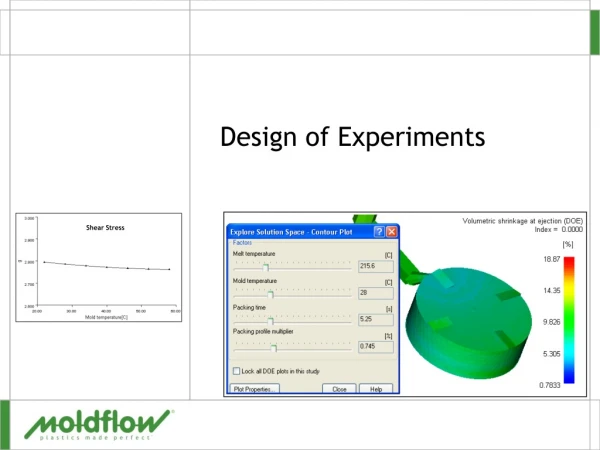
Stat>DOE>Factorial>Create Factorial Design Full Factorial 3 factors Number of replicates
Data for the Fill Height Problem(Average deviation from target in tenths of an inch)
Enter Information Ask for random runs
I don’t want to do all of the math Can I get Minitab to do it for me? Yes, but first let’s look at the results from Minitab and talk about what we get. Then you can have class time to use the screen shots to analyze.
The Pareto Chart shows the significant effects. Anything to the right of the red line is significant at a (1-a) level. In our case a =0.05, so we are looking for significant effects at the 0.95 or 95% confidence level. So what is significant here?
Estimated Effects and Coefficients for Deviation from Target (coded units) Term Effect Coef SE Coef T P Constant 1.0000 0.1976 5.06 0.001 %Carbonation 3.0000 1.5000 0.1976 7.59 0.000 Pressure 2.2500 1.1250 0.1976 5.69 0.000 Line Speed 1.7500 0.8750 0.1976 4.43 0.002 %Carbonation*Pressure 0.7500 0.3750 0.1976 1.90 0.094 %Carbonation*Line Speed 0.2500 0.1250 0.1976 0.63 0.545 Pressure*Line Speed 0.5000 0.2500 0.1976 1.26 0.242 %Carb*Press*Line Speed 0.5000 0.2500 0.1976 1.26 0.242 S = 0.790569 PRESS = 20 R-Sq = 93.59% R-Sq(pred) = 74.36% R-Sq(adj) = 87.98% We could construct an equation from this to predict Deviation from Target. Deviation = 1.00 + 1.50*(%Carbonation) +1.125*(Pressure) + 0.875*(Line Speed) + 0.375*(%Carbonation*Pressure) + 0.125*(%Carbonation*Line Speed) + 0.250*(Pressure*Line Speed) + 0.250*(%Carbonation*Pressure*Line Speed) We can actually get a better model, which we will discuss in a few slides.
Estimated Effects and Coefficients for Deviation from Target (coded units) Term Effect Coef SE Coef T P Constant 1.0000 0.1976 5.06 0.001 %Carbonation 3.0000 1.5000 0.1976 7.59 0.000 Pressure 2.2500 1.1250 0.1976 5.69 0.000 Line Speed 1.7500 0.8750 0.1976 4.43 0.002 %Carbonation*Pressure 0.7500 0.3750 0.1976 1.90 0.094 %Carbonation*Line Speed 0.2500 0.1250 0.1976 0.63 0.545 Pressure*Line Speed 0.5000 0.2500 0.1976 1.26 0.242 %Carb*Press*Line Speed 0.5000 0.2500 0.1976 1.26 0.242 S = 0.790569 PRESS = 20 R-Sq = 93.59% R-Sq(pred) = 74.36% R-Sq(adj) = 87.98% The statisticians at Cummins suggest that you remove all terms that have a p value greater than 0.2. This allows you to have more data to estimate the values of the coefficients.
Here is the final model from Minitab with the appropriate terms. Estimated Effects and Coefficients for Deviation from Target (coded units) Term Effect Coef SE Coef T P Constant 1.0000 0.2030 4.93 0.000 %Carbonation 3.0000 1.5000 0.2030 7.39 0.000 Pressure 2.2500 1.1250 0.2030 5.54 0.000 Line Speed 1.7500 0.8750 0.2030 4.31 0.001 %Carbon*Press 0.7500 0.3750 0.2030 1.85 0.092 S = 0.811844 PRESS = 15.3388 R-Sq = 90.71% R-Sq(pred) = 80.33% R-Sq(adj) = 87.33% Deviation from Target = 1.000 + 1.5*(%Carbonation) + 1.125*(Pressure) + 0.875*(Line Speed) + 0.375*(%Carbonation*Pressure)
>Stat>DOE>Factorial>Analyze Factorial Design Select the Graphs tab to get the next screen
The Pareto Chart shows the significant effects. Anything to the right of the red line is significant at a (1-a) level. In our case a =0.05, so we are looking for significant effects at the 0.95 or 95% confidence level. So what is significant here?
Estimated Effects and Coefficients for Deviation from Target (coded units) Term Effect Coef SE Coef T P Constant 1.0000 0.1976 5.06 0.001 %Carbonation 3.0000 1.5000 0.1976 7.59 0.000 Pressure 2.2500 1.1250 0.1976 5.69 0.000 Line Speed 1.7500 0.8750 0.1976 4.43 0.002 %Carbonation*Pressure 0.7500 0.3750 0.1976 1.90 0.094 %Carbonation*Line Speed 0.2500 0.1250 0.1976 0.63 0.545 Pressure*Line Speed 0.5000 0.2500 0.1976 1.26 0.242 %Carb*Press*Line Speed 0.5000 0.2500 0.1976 1.26 0.242 S = 0.790569 PRESS = 20 R-Sq = 93.59% R-Sq(pred) = 74.36% R-Sq(adj) = 87.98% We could construct an equation from this to predict Deviation from Target. Deviation = 1.00 + 1.50*(%Carbonation) +1.125*(Pressure) + 0.875*(Line Speed) + 0.375*(%Carbonation*Pressure) + 0.125*(%Carbonation*Line Speed) + 0.250*(Pressure*Line Speed) + 0.250*(%Carbonation*Pressure*Line Speed) We can actually get a better model, which we will discuss in a few slides.
>Stat>DOE>Factorial>Factorial Plots Go to set up
Practical Application • Carbonation has a large effect, so try to control the temperature more precisely • There is less deviation at low pressure, so use the low pressure • Although the slower line speed yields slightly less deviation, the process engineers decided to go ahead with the higher line speed - WHY???
We can also use Minitab to construct a predictive model!! Estimated Effects and Coefficients for Deviation from Target (coded units) Term Effect Coef SE Coef T P Constant 1.0000 0.1976 5.06 0.001 %Carbonation 3.0000 1.5000 0.1976 7.59 0.000 Pressure 2.2500 1.1250 0.1976 5.69 0.000 Line Speed 1.7500 0.8750 0.1976 4.43 0.002 %Carbonation*Pressure 0.7500 0.3750 0.1976 1.90 0.094 %Carbonation*Line Speed 0.2500 0.1250 0.1976 0.63 0.545 Pressure*Line Speed 0.5000 0.2500 0.1976 1.26 0.242 %Carb*Press*Line Speed 0.5000 0.2500 0.1976 1.26 0.242 S = 0.790569 PRESS = 20 R-Sq = 93.59% R-Sq(pred) = 74.36% R-Sq(adj) = 87.98% It is recommended to delete items with P > 0.200
>Stat>DOE>Factorial>Analyze Factorial Design Select this arrow to remove the AC, the 2-way interaction with the highest p value.
Estimated Effects and Coefficients for Deviation from Target (coded units) Estimated Effects and Coefficients for Deviation (tenths of inch) (coded units) Term Effect Coef SE CoefT P Constant 1.0000 0.1909 5.24 0.001 %Carbonation 3.0000 1.5000 0.1909 7.86 0.000 Pressure (psi) 2.2500 1.1250 0.1909 5.89 0.000 Line Speed (bpm) 1.7500 0.8750 0.1909 4.58 0.001 %Carbonation*Pressure (psi) 0.7500 0.3750 0.1909 1.96 0.081 Pressure (psi)*Line Speed (bpm) 0.5000 0.2500 0.1909 1.31 0.223 %Carb*Pressure (psi)* 0.5000 0.2500 0.1909 1.31 0.223 Line Speed (bpm) S = 0.763763 PRESS = 16.5926 R-Sq = 93.27% R-Sq(pred) = 78.73% R-Sq(adj) = 88.78% Next term to remove
Here is the final model from Minitab with the appropriate terms. Estimated Effects and Coefficients for Deviation from Target (coded units) Term Effect Coef SE Coef T P Constant 1.0000 0.2030 4.93 0.000 %Carbonation 3.0000 1.5000 0.2030 7.39 0.000 Pressure 2.2500 1.1250 0.2030 5.54 0.000 Line Speed 1.7500 0.8750 0.2030 4.31 0.001 %Carbon*Press 0.7500 0.3750 0.2030 1.85 0.092 S = 0.811844 PRESS = 15.3388 R-Sq = 90.71% R-Sq(pred) = 80.33% R-Sq(adj) = 87.33% Deviation from Target = 1.000 + 1.5*(%Carbonation) + 1.125*(Pressure) + 0.875*(Line Speed) + 0.375*(%Carbonation*Pressure)
Estimated Effects and Coefficients for Deviation from Target (coded units). The term coded units means that the equation uses a -1 for the low value and a +1 for the high value of the data. Deviation from Target = 1.000 + 1.5*(%Carbonation) + 1.125*(Pressure) + 0.875*(Line Speed) + 0.375*(%Carbonation*Pressure) Let’s check this for %Carbonation = 10, Pressure = 30 psi, and Line Speed = 200 BPM %Carbonation is at its low value, so it gets a -1. Pressure is at its high value, so it gets +1, Line Speed is at its low value, so it gets a -1. Deviation from Target = 1.000 + 1.5*(-1) + 1.125*(1)+ 0.875*(-1)+ 0.375*(-1*-1) Deviation from Target = -0.625 tenths of an inch How does this compare with the actual runs at those settings?
>Stat>DOE>Factorial>Response Optimizer Now that we have our model, we can play with it to find items of interest. Select C8 Deviation (tenths of an inch)