Design of Experiments (DOE)
280 likes | 543 Vues
Design of Experiments (DOE). ME 470 Fall 2013 – Day 2. We will use statistics to make good design decisions!.

Design of Experiments (DOE)
E N D
Presentation Transcript
Design of Experiments (DOE) ME 470 Fall 2013 – Day 2
We will use statistics to make good design decisions! We may be forced to run experiments to characterize our system. We will use valid statistical tools such as Linear Regression, DOE, and Robust Design methods to help us make those characterizations.
DOE is a powerful tool for analyzing and predicting system behavior. • At the end of the DOE module, students should be able to perform the following actions: • Explain the advantages of designed experiments (DOE) over one-factor-at-a-time • Define key terminology used in experimental design • Analyze experimental data using the DOE techniques introduced • Make good design decisions!!!
Be prepared to define the terms below. • Factor - A controllable experimental variable thought to influence response (in the case of the Frisbee thrower: angle, motor speed, tire pressure) • Response - The outcome or result; what you are measuring (distance Frisbee goes) • Levels - Specific value of the factor (15 degrees vs. 30 degrees) • Interaction - Factors may not be independent, therefore combinations of factors may be important. Note that these interactions can easily be missed in a straight “hold all other variables constant” scientific approach. If you have interaction effects you can NOT find the global optimum using the “OFAT” (one factor at a time) approach! • Replicate – performance of the basic experiment
There are six suggested steps in DOE. 1. Statement of the Problem 2. Selection of Response Variable 3. Choice of Factors and Levels • Factors are the potential design parameters, such as angle or tire pressure • Levels are the range of values for the factors, 15 degrees or 30 degrees 4. Choice of Design • screening tests • response prediction • factor interaction 5. Perform Experiment 6. Data Analysis
23 Factorial Design Example • #1. Problem Statement: A soft drink bottler is interested in obtaining more uniform heights in the bottles produced by his manufacturing process. The filling machine theoretically fills each bottle to the correct target height, but in practice, there is variation around this target, and the bottler would like to understand better the sources of this variability and eventually reduce it. • #2. Selection of Response Variable: Variation of height of liquid from target • #3. Choice of Factors: The process engineer can control three variables during the filling process: • (A) Percent Carbonation • (B) Operating Pressure • (C) Line Speed • Pressure and speed are easy to control, but the percent carbonation is more difficult to control during actual manufacturing because it varies with product temperature. It can be controlled in a lab setting.
23 Factorial Design Example • #3. Choice of Levels – Each test will be performed for both high and low levels • #4. Choice of Design – Interaction effects • #5. Perform Experiment • Determine what tests are required using tabular data or Minitab • Determine the order in which the tests should be performed
Stat>DOE>Factorial>Create Factorial Design Full Factorial 3 factors Number of replicates
Enter Information Ask for random runs
The Pareto Chart shows the significant effects. Anything to the right of the red line is significant at a (1-a) level. In our case a =0.05, so we are looking for significant effects at the 0.95 or 95% confidence level. So what is significant here?
Estimated Effects and Coefficients for Deviation from Target (coded units) Term Effect Coef SE Coef T P Constant 1.0000 0.1976 5.06 0.001 %Carbonation 3.0000 1.5000 0.1976 7.59 0.000 Pressure 2.2500 1.1250 0.1976 5.69 0.000 Line Speed 1.7500 0.8750 0.1976 4.43 0.002 %Carbonation*Pressure 0.7500 0.3750 0.1976 1.90 0.094 %Carbonation*Line Speed 0.2500 0.1250 0.1976 0.63 0.545 Pressure*Line Speed 0.5000 0.2500 0.1976 1.26 0.242 %Carb*Press*Line Speed 0.5000 0.2500 0.1976 1.26 0.242 S = 0.790569 PRESS = 20 R-Sq = 93.59% R-Sq(pred) = 74.36% R-Sq(adj) = 87.98% We could construct an equation from this to predict Deviation from Target. Deviation = 1.00 + 1.50*(%Carbonation) +1.125*(Pressure) + 0.875*(Line Speed) + 0.375*(%Carbonation*Pressure) + 0.125*(%Carbonation*Line Speed) + 0.250*(Pressure*Line Speed) + 0.250*(%Carbonation*Pressure*Line Speed) We can actually get a better model, which we will discuss in a few slides.
Estimated Effects and Coefficients for Deviation from Target (coded units) Term Effect Coef SE Coef T P Constant 1.0000 0.1976 5.06 0.001 %Carbonation 3.0000 1.5000 0.1976 7.59 0.000 Pressure 2.2500 1.1250 0.1976 5.69 0.000 Line Speed 1.7500 0.8750 0.1976 4.43 0.002 %Carbonation*Pressure 0.7500 0.3750 0.1976 1.90 0.094 %Carbonation*Line Speed 0.2500 0.1250 0.1976 0.63 0.545 Pressure*Line Speed 0.5000 0.2500 0.1976 1.26 0.242 %Carb*Press*Line Speed 0.5000 0.2500 0.1976 1.26 0.242 S = 0.790569 PRESS = 20 R-Sq = 93.59% R-Sq(pred) = 74.36% R-Sq(adj) = 87.98% The statisticians at Cummins suggest that you remove all terms that have a p value greater than 0.2. This allows you to have more data to estimate the values of the coefficients.
Here is the final model from Minitab with the appropriate terms. Estimated Effects and Coefficients for Deviation from Target (coded units) Term Effect Coef SE Coef T P Constant 1.0000 0.2030 4.93 0.000 %Carbonation 3.0000 1.5000 0.2030 7.39 0.000 Pressure 2.2500 1.1250 0.2030 5.54 0.000 Line Speed 1.7500 0.8750 0.2030 4.31 0.001 %Carbon*Press 0.7500 0.3750 0.2030 1.85 0.092 S = 0.811844 PRESS = 15.3388 R-Sq = 90.71% R-Sq(pred) = 80.33% R-Sq(adj) = 87.33% Deviation from Target = 1.000 + 1.5*(%Carbonation) + 1.125*(Pressure) + 0.875*(Line Speed) + 0.375*(%Carbonation*Pressure)
Estimated Effects and Coefficients for Deviation from Target (coded units). The term coded units means that the equation uses a -1 for the low value and a +1 for the high value of the data. Deviation from Target = 1.000 + 1.5*(%Carbonation) + 1.125*(Pressure) + 0.875*(Line Speed) + 0.375*(%Carbonation*Pressure) Let’s check this for %Carbonation = 10, Pressure = 30 psi, and Line Speed = 200 BPM %Carbonation is at its low value, so it gets a -1. Pressure is at its high value, so it gets +1, Line Speed is at its low value, so it gets a -1. Deviation from Target = 1.000 + 1.5*(-1) + 1.125*(1)+ 0.875*(-1)+ 0.375*(-1*-1) Deviation from Target = -0.625 tenths of an inch How does this compare with the actual runs at those settings?
>Stat>DOE>Factorial>Response Optimizer Now that we have our model, we can play with it to find items of interest. Select C8 Deviation (tenths of an inch)
The engineer wants the higher line speed and decides to put the target slightly negative. Why?? NEVER GIVE THIS SETTING TO PRODUCTION UNTIL YOU HAVE VERIFIED THE MODEL!!!
Lawn Mower Example VOC Not too Noisy System Spec Noise Level < 75 db Engine Noise Blade Assy Noise Combustion Noise Blade Speed Muffler Noise Blade Area Blade Width Muffler Volume Blade Length Hole Area Grass Height Diameter Blade to Hsg Clearance
Let’s revisit the Frisbee Thrower and see what the data shows us.
Factorial Fit: Distance (ft versus Speed %, Tire Pressure, Angle (Degrees) Estimated Effects and Coefficients for Distance (ft) (coded units) Term Effect Coef SE Coef T P Constant 51.775 0.9604 53.91 0.000 Speed % 6.000 3.000 0.9604 3.12 0.014 Tire Pressure (psi) -3.125 -1.562 0.9604 -1.63 0.142 Angle (Degrees) -15.650 -7.825 0.9604 -8.15 0.000 Speed %*Tire Pressure (psi) -5.225 -2.612 0.9604 -2.72 0.026 Speed %*Angle (Degrees) -4.400 -2.200 0.9604 -2.29 0.051 Tire Pressure (psi)*Angle (Degrees) 0.075 0.037 0.9604 0.04 0.970 Speed %*Tire Pressure (psi)* 1.775 0.887 0.9604 0.92 0.382 Angle (Degrees) S = 3.84171 PRESS = 472.28 R-Sq = 92.02% R-Sq(pred) = 68.09% R-Sq(adj) = 85.04%
Following recommended procedures, we achieved a reduced model.
Let’s look at both main effects and interaction effects. STAT >DOE>FACTORIAL>FACTORIAL PLOTS