The Finite Difference Method
The Finite Difference Method.

The Finite Difference Method
E N D
Presentation Transcript
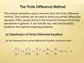
The Finite Difference Method This section presents a quick overview bout the finite difference method. This method can be used to solve any partial differential equation (PDE) usually found in the financial literature of pricing derivatives in general. It can handle very well free boundary problems and optimal stopping problems. (a) Classification of Partial Differential Equations Let the following linear partial differential equation of second order:
where a, b, c, d, e, f and g can be functions of both the independent (x or y), or dependent (u) variable. This equation is of: • parabolic type if b2 - 4ac = 0; • elipic if b2 - 4ac < 0; and • hiperbolic if b2 - 4ac > 0. It is important to note that the majority of the equations found in the financial literature including exotic options and more sophisticated derivatives, are of parabolic type in one dimention (Black-Scholes equation - one state variable plus time). However, in Real Option framework we also find eliptic type as well as parabolic type in one or two dimentions (two state variables plus time). It is important to note that Finite Difference Method are capable of evaluating any type of linear and non-linear Partial Differential Equation as well as Ordinary Differential Equations .
(b) The Finite Difference Method The finite Different Method (FDM) consists of transforming the partial derivatives in difference equations over a small interval. Assuming that u is function of the independent variables x and y , we can divided the x-y plan in mesh points equal to dx = h e dy = k, as showed bellow :
We can evaluate u at point P by : uP = u(ih,jk) = ui,j The value of the second derivative at P could also be evaluated by:
The value of the first derivative at P can be evaluated by three approximations: 1) Central difference:
2) Forward difference: 3) Backward difference:
(c) Explicit Method ´ Implicit Method in a PDE of Parabolic type After substituting the derivatives approximations over the PDE, PDE is corverted into a set of finite difference equations that can be solved either by explicit or implicit method. From now on we will think of the j index as time to expiration (so that j + 1 means more time to expiration, an earlier time instant), and i index as price. Explicit method allows to evaluate the unknown value today ui,j+1 directly from the subsequent known future values ui-1,j, ui,j and ui+1,j. It can be done because we have proper boundary conditions that always set any values at the termination date. It can be viewd as well as a dynamic programming backward procedure. Therefore the application of explicit method leads to a difference equation as follow:
The molecule of a PDE using the explicit method is represented bellow. Unknown value is in red and known values in black: Implicit method does not allow a directly approach to evaluate the unknown value. Instead of we found an expression as follows: The molecule of a PDE using the implicit method is represented bellow. Unknown values is in red and known value in black:
Therefore we have to solve a silmutaneous system of linear equations to evaluate the unknow values.
Supose the parabolic PDE already has been transformed in a set of difference equations. We obtain the following grid where red terms remains to be evaluated.
Using the explicit method, the elements u1 - u9 can be evaluated direclty over the subsequent elements, which are the boundary condition 1.
However, if we were using the implicit method we will have a system of 9 simultaneous linear equations, and obtain the 9 unknown values simultaneously.
(d) Convergence and Stability Implicit method is always stable. Nonetheless, explicit method has to be carefully employed. For parabolic PDE, after substituting the derivatives by its approximations, it leads to the following difference equation: A quick way to guarantee the convergence and stability is set a, b and c > 0 by changing the interval lenght in discretization process.