Delaunay Triangulation (DT)
Delaunay Triangulation (DT). Lehrstuhl für Informatik 10 (Systemsimulation) Ruslana Mys. Introduction Delaunay-Voronoi based method Algorithms to compute the convex hull Algorithms for generating the DT Conclusion. Two basic types of the mesh. Unstructured mesh. Structured mesh.

Delaunay Triangulation (DT)
E N D
Presentation Transcript
Delaunay Triangulation (DT) Lehrstuhl für Informatik 10 (Systemsimulation) Ruslana Mys • Introduction • Delaunay-Voronoi based method • Algorithms to compute the convex hull • Algorithms for generating the DT • Conclusion
Two basic types of the mesh Unstructured mesh Structured mesh Introduction
Structured Meshes Unstructured Meshes Multiblock Approaches Hybrid Approache Outline of mesh generation approches Introduction
The Delaunay triangulation is closely related geometrically to the Voronoi tessellation (also known as the Direchlet or Theissen tessellations). Voronoi diagram
The Delaunay triangulation is created by connecting all generating points which share a common tile edge. Thus formed, the triangle edges are perpendicular bisectors of the tile edges. This method has the O(log(n)) complexity. Voronoi diagram
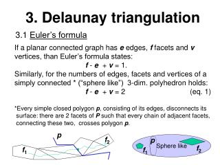
The E satisfies min-max angle property iff either the quadrilateral formed by the two triangles sharing edge E is not strictly convex, or E is the diagonal of quadrilateral which maximizes the minimum of the six internal angles associated with each of the two possible triangulations of quadrilateral. E E Non-convex quadrilateral Maximization Maximum-Minimum Angle Property
Let E be an internal edge of triangulation. Then E satisfies local empty-circle property iff the circumcircle of any of two triangles sharing edge E does not contain the vertex of the other triangle in ist interior. E E Not Delaunay triangulation Delaunay triangulation Local Empty-Circle Property
Algorithms to computing the convex hull of set of points: • Incremental and Gift wrapping algorithms the idea is to add the points one at a time updating the hull first step is to compute the area A of starting triangle as where xi and yi are the coordinates of trianglevertecies (in 2D) • Divide and conquer algorithm O(n*log(n))) can be used if the domain is very large If A ≤ 0 → incremental algorithm (the points occure inclockwise order) O(n2) If A ≥ 0 → gift wrapping algorithm (the pointsoccure in anti-clockwise order) (if the # of sides of the hull is h, then O(nh)) Algorithms to computing the convex hull
Incremental and Gift wrapping algorithms: • Incremental • Delete all edges from the hull that the new point can see • Add two edges to connect the new point to the remainder of the old hull • Repeat for the next point outside the hull • Gift wrapping • Find least point A (with minimum y-coordinate) as the starting point • We can find B where all points lie to the left of AB by scanning through all the points • Similarly, we can find C where all points lie to the left of BC and so on Algorithms to computing the convex hull
First sort the points by x coordinate Divide the points into two equal sized sets L and R s.t. all points of L are to the left of the most leftmost points in R. Recursively find the convex hull of L and R Divide and conquer algorithm: O(log(n)) • 2D-case Algorithms to computing the convex hull
Divide and conquer algorithm: • To merge the left hull and the right hull it is necessary to find the two red edges • The upper common tangent can be found in linear time by scanning around the left hull in a clockwise direction and around the right hull in an anti-clockwise direction • The two tangents divide each hull into two pieces. The edges belonging to one of these pieces must be deleted Algorithms to computing the convex hull
Divide and conquer algorithm: • 3D-case • To merge in 3D need to construct a cylinder of triangles connecting the left hull and the right hull • One edge of the cylinder AB is just the lower common tangent which can be computed just as in the 2D case Algorithms to computing the convex hull
Divide and conquer algorithm: • Next need to find a triangle ABC belonging to the cylinder which has AB as one of its edges. The third vertex of the triangle (C) must belong to either the left hull or the right hull. (In this case it belongs to the right hull) • After finding triangle ABC we now have a new edge AC that joins the left hull and the right hull. We can find triangle ACD just as we did ABC. Continuing in this way, we can find all the triangles belonging to the cylinder, ending when we get back to AB. Algorithms to computing the convex hull
Algorithms to generate the DT: • Two-steps algorithm • Computation of an arbitrary triangulation • Optimization of triangulation to produce a Delaunay triangulation O(n2) O(n2) • Incremental (Watson’s) algorithm • Modification of an existing Delaunay triangulation while adding anew vertex at a time • Sloan‘s algorithm • Computation of Delaunay triangulation of arbitrary domain Algorithms for genereting the (DT)
Two-steps algorithm: Used to produce the coarse triangulation in refinement simplification process • Computation of an any arbitrary triangulation of domain • Optimaze this triangulation to produce the DT Optimization step: for every internal edge E do • If E is not locally optimal, then swap it with the other diagonal of the quadrilateral formed by the two triangles sharing edge E • Repeat the previose loop until one pass through the whole loop does not cause any edge swap Algorithms for generating the DT
Optimization step: An edge pq is locally optimal iff • Point s in the plane is outside circle prq • Point l(s) in 3D space is above the oriented plane defined by the triple l(p), l(r) , l(q) Algorithms for generating the DT
Optimization step: An edge pq is not locally optimal (it must be swapped) iff • Point s in the plane is inside circle prq • Point l(s) in 3D space is below the oriented plane defined by the triple l(p), l(r), l(q) Algorithms for generating the DT
Incremental (Watson’s) algorithm: • Detection of the influence region • Deletion of the triangles of this region • Re-triangulate the region by join the point to the verticies of the influence polygon Algorithms for generating the DT
Incremental (Watson’s) algorithm: After 100 insertion Initial triangulation After 200 insertion After 314 insertion Algorithms for generating the DT
7 4 3 1 2 5 6 Sloan’s algorithm: • Nodalization of the domain • Form a supertriangle by tree points, which is completely encompasses all points to be triangulated • Create a triangle list array T, where the supertriangle is listed as the first triangle • Introduce the first point into the supertriangle and generate three triangles by connecting the three vertices of the supertriangle • Delete the supertiangle from the list and put there three newly formed triangles Algorithms for generating the DT
7 4 3 1 2 5 6 7 4 3 1 2 5 6 Sloan’s algorithm: • Introduce the next point for triangulation • Optimize the grid • Repeat the previous two steps until all N points are consumed • Finally, all triangles, which contain one or more of the vertices of supertriangle, are removed Algorithms for generating the DT
Advantages of DT: • Wide range of utilization • Irregular connectivity • Number of neighboring nodes variable • Equally easy (or difficult!) to generate for all domains • Easy to vary point density • Automatic mesh generation • Elegant theoretical foundations • Inherent grid quality (Dis)advantages of DT: • Maximizes minimum angle in 2D, not in 3D • Does not preserve original surface mesh • Can produce sliver elements at the boundary Conclusion
Thank you for your attention ! Thank you for your attention !