Choosing the “most probable state path”
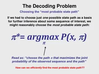
The Decoding Problem . Choosing the “most probable state path”. If we had to choose just one possible state path as a basis for further inference about some sequence of interest, we might reasonably choose the most probable state path : . p * = argmax P(x, p ). p.

Choosing the “most probable state path”
E N D
Presentation Transcript
The Decoding Problem Choosing the “most probable state path” If we had to choose just one possible state path as a basis for further inference about some sequence of interest, we might reasonably choose the most probable state path: p*= argmax P(x, p) p Read as: “choose the path p that maximizes the joint probability of the observed sequence and the path” How can we efficiently find the most probable state path??
Runtime of algorithms “Big O” notation – an upper bound on asymptotic growth • Order • O(c) • O(log n) • O(n) • O(n log n) • O(n2) • O(nc) c>1 • O(cn) c>1 • O(n!) • Name • Constant • Log • Linear • Loglinear • Quadratic • Polynomial • Exponential • Factorial In the context of problems related to sequences, n usually corresponds to the sequence length (which we often designate L)
Runtime of algorithms “Big O” notation – an upper bound on asymptotic growth Image from http://www.cs.odu.edu/~toida/nerzic/content/function/growth.html • O(c) • O(log n) • O(n) • O(n log n) • O(n2) • O(nc) c>1 • O(cn) c>1 • O(n!) Polynomial problems are tractable for reasonable c, but problems with superpolynomial runtime are intractable except for surprisingly small n
Most Probable State Path A naïve approach might recursively explore all possible paths 0 1 2 3 4 The naïve approach ends up solving the same subproblem (and subproblems of those subproblems) numerous times!
The Viterbi Algorithm The Viterbi algorithm is a standard method for finding the most probable state path “The Viterbi variable for state k at position i” vk(i) = P(x1…xi , p*i = k) “the probability of the sequence from the beginning to the symbol at position i, requiring that the most probable partial path ending with state k at position i” This time, let’s look at a practical example of Viterbi in action before getting carried away with an attempt to formalize the equations
The Viterbi Algorithm Finding the most probable state path S Candidate Best paths 0.1 0.9 A: 0.30 A: 0.20 0.5 C: 0.35 C: 0.25 G: 0.25 G: 0.15 T: 0.30 T: 0.20 0.5 0.4 0.6 State “+” State “-” _ A C G 1 · 0.1· 0.3 0 · 0.5· 0.3 0 ·0.6· 0.3 0.03 1 0 0 The parameters shown here are highly artificial and intended to favour state switching
The Viterbi Algorithm Finding the most probable state path S Candidate Best paths 0.1 0.9 A: 0.20 A: 0.30 0.5 C: 0.25 C: 0.35 S S G: 0.25 G: 0.15 T: 0.20 T: 0.30 0.5 0.4 0.6 State “+” State “-” _ A C G 0.03 1 0 0 1 · 0.9· 0.2 0 · 0.5· 0.2 0 ·0.4· 0.2 0.18 The parameters shown here are highly artificial and intended to favour state switching
The Viterbi Algorithm Finding the most probable state path S Candidate Best paths 0.1 0.9 A: 0.20 A: 0.30 0.5 C: 0.35 C: 0.25 ← - S S G: 0.15 G: 0.25 T: 0.20 T: 0.30 0.5 0.4 0.6 State “+” State “-” _ A C G 0.03 · 0.5· 0.25 0.18 · 0.6· 0.25 0.03 0.027 0 1 0 0.18 The parameters shown here are highly artificial and intended to favour state switching
The Viterbi Algorithm Finding the most probable state path S Candidate Best paths 0.1 0.9 A: 0.30 A: 0.20 0.5 C: 0.25 C: 0.35 ← - S S G: 0.15 G: 0.25 T: 0.20 T: 0.30 ← - 0.5 0.4 0.6 State “+” State “-” _ A C G 0.03 0.027 0.03 · 0.5· 0.35 0.18 · 0.4· 0.35 0 1 0 0.18 0.0252 The parameters shown here are highly artificial and intended to favour state switching
The Viterbi Algorithm Finding the most probable state path S Candidate Best paths 0.1 0.9 A: 0.20 A: 0.30 0.5 C: 0.35 C: 0.25 ← - ← + S S G: 0.25 G: 0.15 T: 0.30 T: 0.20 ← - 0.5 0.4 0.6 State “+” State “-” _ A C G 0.03 0.027 0.002268 0.0270· 0.5· 0.15 0.0252· 0.6· 0.15 0 1 0 0.18 0.0252 The parameters shown here are highly artificial and intended to favour state switching
The Viterbi Algorithm Finding the most probable state path S Candidate Best paths 0.1 0.9 A: 0.30 A: 0.20 0.5 C: 0.25 C: 0.35 ← - ← + ← + S S G: 0.15 G: 0.25 T: 0.20 T: 0.30 ← + ← - ← - 0.5 0.4 0.6 State “+” State “-” _ A C G 0.0270· 0.5· 0.25 0.0252· 0.4· 0.25 0.03 0.027 0.002268 1 0 0 0.18 0.003375 0.0252 The parameters shown here are highly artificial and intended to favour state switching
The Viterbi Algorithm The Viterbi algorithm is the standard method for finding the most probable state path “The Viterbi variable for state k at position i” vk(i) = P(x1…xi , p*i = k) “the probability of the sequence from the beginning to the symbol at position i, requiring the most probable partial path ending with state k at position i” Did the example illustrate how this helps?
The Viterbi Algorithm A recursive definition for Viterbi variables vk(i) = P(x1…xi , p*i = k) Again, we recursively define the Viterbi variables in terms of their own values at prior positions in the sequence… vl(i+1) = el(xi+1 ) max (vk(i) k Note that a maximization step replaces the summation across states that we had in the forward algorithm. Termination is again assured by the fact that all paths must begin with Start Equations of this latter form are sometimes known as Bellman equations.
The Viterbi Algorithm What if we had in our possession all of the Viterbi variables for L, the last position of the sequence? This term disappears if ends are not modelled! P(x,p*) = That would be very useful indeed, since to get the probability of the observed sequence and the most probable state path we would need only ask which state k was associated with the maximum-valued Viterbi variable at the final position • Two problems: • We don’t yet know those “final position” Viterbi variables • This doesn’t tell us what the state path actually was...
The Viterbi Algorithm Putting it all together • Initialization: • vstart(0) = 1 andvk(0) = 0 for all other initial states k Recursion (i = 1 … L): vl(i) = el(xi) ptri(l)= Termination: P(x,p*) = pL*= Traceback (i = L .. 1): p*i-1=ptr𝒊(p𝒊∗) Note the similarity to forward, but with the addition of a traceback
The Viterbi Algorithm Reduction to Python code The max function, along with list comprehensions might come in handy for certain parts of your Viterbi implementation. For instance, here’s a one-liner that fulfills the termination conditions and uses both language features: return ( max ( [(vtable[self.sequence_length][state], possible_paths[state]) for state in self.transitions)] ) List comprehensions perform iterative operations on lists, and result in new lists. Here, the probability and the path list are handled together as a tuple. The max function will operate on just the first element in a tuple, so the state path “comes along for the ride”
Dynamic Programming An anecdote from Richard Bellman “I spent the Fall quarter (of 1950) at RAND. My first task was to find a name for multistage decision processes. An interesting question is, Where did the name, dynamic programming, come from? The 1950s were not good years for mathematical research. We had a very interesting gentleman in Washington named Wilson. He was Secretary of Defense, and he actually had a pathological fear and hatred of the word, research. I’m not using the term lightly; I’m using it precisely. His face would suffuse, he would turn red, and he would get violent if people used the term, research, in his presence. You can imagine how he felt, then, about the term, mathematical. The RAND Corporation was employed by the Air Force, and the Air Force had Wilson as its boss, essentially. Hence, I felt I had to do something to shield Wilson and the Air Force from the fact that I was really doing mathematics inside the RAND Corporation. What title, what name, could I choose? In the first place I was interested in planning, in decision making, in thinking. But planning, is not a good word for various reasons. I decided therefore to use the word, “programming” I wanted to get across the idea that this was dynamic, this was multistage, this was time-varying I thought, lets kill two birds with one stone. Lets take a word that has an absolutely precise meaning, namely dynamic, in the classical physical sense. It also has a very interesting property as an adjective, and that is its impossible to use the word, dynamic, in a pejorative sense. Try thinking of some combination that will possibly give it a pejorative meaning. Its impossible. Thus, I thought dynamic programming was a good name. It was something not even a Congressman could object to. So I used it as an umbrella for my activities” Excerpt from Richard Bellman “Eye of the Hurricane: an autobiography”, 1984
Dynamic Programming Dynamic programming algorithms solve problems by solving simpler subproblems and storing and reusing these subsolutions What kinds of problems are solved with dynamic programming? • The problem must have the property of an optimal substructure. • Having an optimal substructure means that an optimal solution can be constructed efficiently from optimal solutions of its subproblems • The problem must have overlappingsubproblems so that we benefit from the storage and reuse of earlier subproblems Why are dynamic programming approaches so common when dealing with DNA or amino acid sequences?
Dynamic Programming A substring of a string is still a string AGCTCAATTAGGAC AGCTCAATTAGGA AGCTCAATTAGG AGCTCAATTAG AGCTCAATTA AGCTCAATT AGCTCAAT AGCTCAA ... A Problems relating to DNA sequences very frequently naturally posses the optimum substructure property
Dynamic Programming Problems relating to biological sequences can often be structured in terms of “overlapping subproblems” AGCTCAAT Biological sequences very often satisfy both the ideal optimal substructure and overlapping subproblem criteria and are therefore natural candidates for dynamic programming approaches
Dynamic Programming Dynamic programming problems often have a natural representation as a trellis-like graph rather than as a tree 0 1 2 3 4 5 6 Start *the direction of arrows shown here corresponds to the possible tracebackpaths, not to the main forward iteration By exploiting the repetitive structure of the problem, dynamic programming converted our most probable state path problem from one with naïve complexity of O(|states|L) to one with complexity O(L ∙ |states|2)
Dynamic Programming General procedure for dynamic programming Characterize the structure of an optimal solution Recursively define the value of an optimal solution Compute the value of an optimal solution in a bottom-up fashion (Optionally) construct the optimal solution from the computed information Can you identify each step in the dynamic programming approach in our descriptions of the forward and the Viterbi algorithms?