Download
1 / 48
480 likes | 567 Vues
This review covers concepts like recursive procedures, pseudocode for algorithms, merge sort, tree properties, induction techniques, and red-black trees. Learn about binary search trees, full binary trees, complete binary trees, height-balanced binary trees, and Red-black tree operations.

E N D
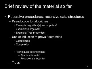
Brief review of the material so far • Recursive procedures, recursive data structures • Pseudocode for algorithms • Example: algorithm(s) to compute an • Example: merge sort • Example: Tree properties • Use of induction to prove / determine • Correctness • Complexity • Techniques to remember: • Structural induction • Recursion and induction • Trees
Exercise Use induction to prove that the number of nodes in a binary tree is at most 2h(T)+1-1 where h(T) is the height of the tree.
Discrete Structures & AlgorithmsEfficient data structures and algorithms(Red-black trees)
A binary search tree (BST) is a binary tree with the following properties: • The key of a node is always greater than the keys of the nodes in its left subtree. • The key of a node is always smaller than the keys of the nodes in its right subtree.
Stored keys must satisfy the binary search tree property. y in left subtree of x, then key[y] key[x]. y in right subtree of x, then key[y] key[x]. 26 200 28 190 213 18 12 24 27 Binary search trees 56
Height of a binary tree • Most BST operations have a time complexity that is related to the height of the tree. • At worst, can be n, where n is the total number of nodes.
A full binary tree • If, for a tree of height h, all levels are full. • All nodes at height (or depth) h are leaf nodes. • How many nodes exist in a full binary tree of height h?
A full binary tree Theorem: A full BST of height h has 2h - 1 nodes Proof: Use induction. Inductive Basis: A tree of height 1 has one node (the root). Inductive Hypothesis: Assume that a tree of height h has 2h - 1 nodes. …
L R h+1 h A full binary tree Inductive step: Connect two trees of height h to make one of height h+1. You need to add one more node for the new root. root By the inductive hypothesis, the new number of nodes is (2h - 1) + (2h - 1) + 1 = 2h+1 - 1 … proved!
Minimum height of a binary tree • We saw that a full binary tree of height h has n=2h-1 nodes. • Given n keys (values), what is the smallest height of a binary tree that can store these n keys? • hmin = 1+log2n • for any real number x, x is the largest integer smaller than or equal to x. • Similarly, x is the smallest integer greater than or equal to x. • Prove as an exercise.
Complete binary trees • A complete binary tree (of height h) satisfies the following conditions: • Level 0 to h-1 represent a fullbinary tree of height h. • One or more nodes in level h-1 may have 0, or 1 child nodes. • If j, k are nodes in level h-1, then j has more child nodes than kif and only ifj is to the left of k.
Complete binary trees • Given a set of n nodes, a complete binary tree of these nodes provides the maximum number of leaves with the minimal average path length (per node). • The complete binary tree containing n nodes must have at least one path from root to leaf of length log n.
Height-balanced binary trees • A height-balanced binary tree is a binary tree such that: • The left and right subtrees for any given node differ in height by no more than one. • Note: A complete binary tree is height-balanced
Time complexity of BST operations • All dynamic-set search operations can be supported in O(h) time. • h = (lg n)for a balanced binary tree (and for an average tree built by adding nodes in random order.) • h = (n) for an unbalanced tree that resembles a linear chain of n nodes in the worst case. It is better to keep the tree balanced.
B L A B M C C A L M Building a BST Is there a unique BST for letters A B C L M ? No!Different input sequences result in different trees. Therefore, we may need to explicitly balance a tree. Inserting:A B C L M Inserting:C A B L M
Keeping the height of a BST small improves the running time of algorithms on the tree.
Red-black trees • “Balanced” binary trees guarantee an O(lg n) running time on the basic dynamic-set operations. • Red-black tree • Binary tree with an additional attribute for its nodes: color which can be red or black. • Constrains the way nodes can be colored on any path from the root to a leaf. • Ensures that no path is more than twice as long as another the tree is ‘balanced’. • The nodes inherit all the other attributes from the binary search trees: key, left, right, p.
Red-black trees A binary search tree where: • Every node is either red or black. • The root is black. • Every leaf (NIL) is black. • If a node is red, then both its children are black. • No two red nodes in a row on a simple path from the root to a leaf. • For each node, all paths from the node to descendant leaves contain the same number of black nodes.
Example: RED-BLACK TREE 26 • For convenience we use a sentinel NIL[T] to represent all the NIL nodes at the leafs • NIL[T] has the same fields as an ordinary node • Color[NIL[T]] = BLACK • The other fields may be set to arbitrary values 17 41 NIL NIL 30 47 38 50 NIL NIL NIL NIL NIL NIL
26 17 41 NIL NIL 30 47 38 50 NIL NIL NIL NIL NIL NIL ‘Black-height’ of a node h = 4 bh = 2 • Height of a node:the number of edges in a longest path to a leaf • Black-height of a node x: bh(x) is the number of black nodes (including NIL) on the path from x to leaf, not counting x. h = 3 bh = 2 h = 1 bh = 1 h = 2 bh = 1 h = 2 bh = 1 h = 1 bh = 1 h = 1 bh = 1
26 17 41 30 47 38 50 Properties of red-black trees (1) • Claim • Any node with height h has black-height >= h/2. • Proof • By property 4, at most h/2 red nodes on the path from the node to a leaf. • Hence at least h/2 are black. • Property 4: if a node is red then both its children are black.
Properties of red-black trees (2) Claim: The subtree rooted at any node x contains at least 2bh(x) - 1 internal nodes. Proof: By induction on height of x. Basis: height[x] = 0 x is a leaf (NIL[T]) bh(x) = 0 # of internal nodes: 20 - 1 = 0 x NIL
26 17 41 30 47 38 50 Properties of red-black trees (2.cont) Inductive step: • Let height(x) = h and bh(x) = b. • Any child y of x has: • bh (y) = • bh (y) = b (if the child is red), or b - 1 (if the child is black)
Properties of red-black trees (2.cont) • Want to prove: • The subtree rooted at any node x contains at least 2bh(x) - 1 internal nodes. • Internal nodes for each child of x: 2bh(x) - 1 - 1. [induction hypothesis] • The subtree rooted at x contains at least: (2bh(x) - 1 – 1) + (2bh(x) - 1 – 1) + 1 = 2 · (2bh(x) - 1 - 1) + 1 = 2bh(x) - 1 internal nodes. x r l
Properties of red-black trees (3) Lemma: A red-black tree with n internal nodes has height at most 2 lg(n + 1). Proof: n • Add 1 to both sides and then take logs: n + 1 ≥ 2b ≥ 2h/2 lg(n + 1) ≥ h/2 h ≤ 2 lg(n + 1) root height(root) = h bh(root) = b r l ≥ 2h/2 - 1 ≥ 2b - 1 number n of internal nodes since b h/2
Operations on red-black trees • The non-modifying binary-search-tree operations MINIMUM, MAXIMUM, SUCCESSOR, PREDECESSOR, and SEARCH run in O(h) time. • They take O(lg n) time on red-black trees. • What about TREE-INSERT and TREE-DELETE? • They will still run on O(lg n). • We have to guarantee that the modified tree will still be a red-black tree.
26 17 41 30 47 38 50 INSERT INSERT: How do we colour the new node? • Red? Let’s insert 35. • Property 4 violated: if a node is red, then both its children are black. • Black? Let’s insert 14. • Property 5 violated: all paths from a node to its leaves contain the same number of black nodes.
Not OK! If removing the root and the child that replaces it is red. 26 Not OK! Could change the black heights of some nodes. Not OK! Could create two red nodes in a row. 17 41 30 47 38 50 DELETE DELETE: What color was the node that was removed? Black? • Every node is either red or black. • The root is black. • Every leaf (NIL) is black. • If a node is red, then both its children are black. • For each node, all paths from the node to descendant leaves contain the same number of black nodes. OK! OK!
Rotations • Operations for restructuring the tree after insert and delete operations on red-black trees. • Rotations take an (almost) red-black-tree and a node within the tree and: • Together with some node re-coloring they help restore the red-black-tree property. • Change some of the pointer structure. • Do not change the binary-search tree property. • Two types of rotations: • Left & right rotations.
Left rotations • Assumptions for a left rotation on a node x: • The right child of x (denoted y) is not NIL; • Root’s parent is NIL. • Idea: • Pivots around the link from x to y; • Makes y the new root of the subtree; • x becomes y’s left child; • y’s left child becomes x’s right child.
LEFT-ROTATE(T, x) • y ← right[x] ►Set y • right[x] ← left[y] ►y’s left subtree becomes x’s right subtree • if left[y] NIL • then p[left[y]] ← x ►Set the parent relation from left[y] to x • p[y] ← p[x] ►The parent of x becomes the parent of y • if p[x] = NIL • then root[T] ← y • else if x = left[p[x]] • then left[p[x]] ← y • else right[p[x]] ← y • left[y] ← x ►Put x on y’s left • p[x] ← y ►y becomes x’s parent
Insertion • Goal: • Insert a new node z into a red-black-tree. • Idea: • Insert node z into the tree as for an ordinary binary search tree; • Color the node red; • Restore the red-black-tree properties. • Use an auxiliary procedure RB-INSERT-FIXUP.
y ← NIL x ← root[T] while x NIL do y ← x if key[z] < key[x] then x ← left[x] else x ← right[x] p[z] ← y Initialize nodes x and y Throughout the algorithm y points to the parent of x. Go down the tree until reaching a leaf; At that point y is the parent of the node to be Inserted. 26 17 41 30 47 Sets the parent of z to be y 38 50 RB-INSERT(T, z)
if y = NIL then root[T] ← z else if key[z] < key[y] then left[y] ← z else right[y] ← z left[z] ← NIL right[z] ← NIL color[z] ← RED RB-INSERT-FIXUP(T, z) The tree was empty: set the new node to be the root. Otherwise, set z to be the left or right child of y, depending on whether the inserted node is smaller or larger than y’s key. 26 17 41 Set the fields of the newly added node. 30 47 Fix any inconsistencies that could have been introduced by adding this new red Node. 38 50 RB-INSERT(T, z)
If p(z) is red not OK. z and p(z) are both red. OK! 26 17 41 38 47 50 Properties affected by insertion OK! • Every node is either red or black. • The root is black. • Every leaf (NIL) is black. • If a node is red, then both its children are black. • For each node, all paths from the node to descendant leaves contain the same number of black nodes. If z is the root not OK. OK!
RB-INSERT-FIXUP – Case 1 z’s “uncle” (y) is red. Idea: (z is a right child) • p[p[z]] (z’s grandparent) must be black: z and p[z] are both red. • Color p[z] black. • Color y black. • Color p[p[z]] red. • Push the “red” violation up the tree • Make z = p[p[z]].
RB-INSERT-FIXUP – Case 1 z’s “uncle” (y) is red. Idea: (z is a left child) • p[p[z]] (z’s grandparent) must be black: z and p[z] are both red. • color[p[z]] black. • color[y] black. • color p[p[z]] red. • z = p[p[z]]. • Push the “red” violation up the tree. Case 1
Case 3 RB-INSERT-FIXUP – Case 3 Idea: • color[p[z]] black. • color[p[p[z]]] red. • RIGHT-ROTATE(T, p[p[z]]). • No longer have 2 reds in a row. • p[z] is now black. Case 3: • z’s “uncle” (y) is black. • z is a left child. Case 3
Case 2 Case 3 RB-INSERT-FIXUP – Case 2 Case 2: • z’s “uncle” (y) is black. • z is a right child. Idea: • z p[z]. • LEFT-ROTATE(T, z). now z is a left child, and both z and p[z] are red Case 3. Case 2
The while loop repeats only when Case 1 is executed: O(lg n) times Set the value of x’s “uncle” We just inserted the root, or The red violation reached the root. RB-INSERT-FIXUP(T, z) • while color[p[z]] = RED do • if p[z] = left[p[p[z]]] • then y ← right[p[p[z]]] • if color[y] = RED • then Case 1 • else if z = right[p[z]] • then Case 2 • else Case 3 • else (same as then clause with “right” and “left” exchanged) • color[root[T]] ← BLACK
Case 1 Case 3 Case 2 11 2 2 14 14 7 7 1 1 15 15 5 5 8 8 4 4 4 7 11 z y 2 11 7 14 z 1 5 8 14 8 2 15 4 15 5 1 Example Insert 4 11 y z y z and p[z] are both red z’s uncle y is red z and p[z] are both red z’s uncle y is black z is a right child z z and p[z] are red z’s uncle y is black z is a left child
Analysis of RB-INSERT • Inserting the new element into the tree O(lg n). • RB-INSERT-FIXUP • The while loop repeats only if CASE 1 is executed. • The number of times the while loop can be executed is O(lg n). • Total running time of RB-INSERT: O(lg n).
Red-black trees - summary • Operations on red-black trees: • SEARCH O(h) • PREDECESSOR O(h) • SUCCESOR O(h) • MINIMUM O(h) • MAXIMUM O(h) • INSERT O(h) • DELETEO(h) • Red-black trees guarantee that the height of the tree will be O(lg n).
Wrap-up • Determining the complexity of algorithms is usually the first step in obtaining better algorithms. • Or realizing we cannot do any better. • What should you know? • Properties of red-black trees. • Proofs for red-black trees. • Operations on red-black trees. • Exploiting invariants and recursive structures in proofs.