Download
1 / 57
1.15k likes | 4.01k Vues
Properties of the OLS Estimator. Quantitative Methods 2 Lecture 5. Edmund Malesky, Ph.D., UCSD. Solutions for β 0 and β 1. OLS Chooses values of β 0 and β 1 that minimizes the unexplained sum of squares. To find minimum take partial derivatives with respect to β 0 and β 1.

E N D
Properties of the OLS Estimator Quantitative Methods 2 Lecture 5 Edmund Malesky, Ph.D., UCSD
Solutions for β0 and β1 • OLS Chooses values of β0 and β1 that minimizes the unexplained sum of squares. • To find minimum take partial derivatives with respect to β0 and β1
Solutions for β0 and β1 • Derivatives were transformed into the normal equations • Solving the normal equations for β0 and β1 gives us our OLS estimators
Solutions for β0 and β1 • Our estimate of the slope of the line is: • And our estimate of the intercept is:
Estimators and the “True” Coefficients • are the “true”coefficients if we only wanted to describe the data we have observed • We are almost ALWAYS using data to draw conclusions about cases outside our data • Thus are estimates of some “true” set of coefficients (β0 and β1) thatexist beyond our observed data
Some Terminology for Labeling Estimators • Various conventions used to distinguish the “true” coefficients from the estimates that we observe. We will use the beta versus beta-hat distinction from Wooldridge. • But other authors, textbooks, or websites may use different terms. Think of this as the same distinction between population values and sample-based estimates
Gauss-Markov Theorem: Under the 5 Gauss-Markov assumptions, the OLS estimator is the best, linear, unbiased estimator of the true parameters (β’s) conditional on the sample values of the explanatory variables. In other words, the OLS estimators is BLUE Karl Freidrich Gauss Andrey Markov
5 Gauss-Markov Assumptions for Simple Linear Model (Wooldridge, p.65) • Linear in Parameters • Random Sampling of n observations • Sample variation in explanatory variables. xi’s are not all the same value • Zero conditional mean. The error u has an expected value of 0, given any values of the explanatory variable • Homoskedasticity. The error has the same variance given any value of the explanatory variable.
The Linearity Assumption • Key to understanding OLS models. • The restriction is that our model of the population must be linear in the parameters. • A model cannot be non-linear in the parameters • Non-linear in the variables (x’s), however, is fine and quite useful
y=ln(x) y 0 1 x
Quadratic Function (y=6+8x-2x2) y 14 6 0 2 x
F(y/x) Demonstration of the Homskedasticity Assumption Predicted Line Drawn Under Homoskedasticity y Variance across values of x is constant x1 x2 x3 x4 x
F(y/x) Demonstration of the Homskedasticity Assumption Predicted Line Drawn Under Heteroskedasticity y Variance differs across values of x x1 x2 x3 x4 x
How Good are the Estimates? Properties of Estimators • Small Sample Properties • True regardless of how much data we have • Most desirable characteristics • Unbiased • Efficient • BLUE (Best Linear Unbiased Estimator)
“Second Best” Properties of Estimators • Asymptotic (or large sample) Properties • True in hypothetical instance of infinite data • In practice applicable if N>50 or so • Asymptotically unbiased • Consistency • Asymptotic efficiency
Bias • A parameter is unbiased if • In other words, the average value of the estimator in repeated sampling equals the true parameter. • Note that whether an estimator is biased or not implies nothing about its dispersion.
Efficiency • We might want to choose a biased estimator, if it has a smaller variance. • An estimator is efficient if its variance is less than any other estimator of the parameter. • This criterion only useful in combination with others. (e.g. =2 is low variance, but biased) is the“best” Unbiased estimator if ,where is any other unbiased estimator of β
F(βx) Unbiased and efficient estimator of β Biased estimator of β High Sampling Variance means inefficient estimator of β 0 β + bias True β
BLUE (Best Linear Unbiased Estimate) • An Estimator is BLUE if: • is a linear function • is unbiased: • is the most efficient:
Large Sample Properties • Asymptotically Unbiased • As n becomes larger E( ) trends toward βj • Consistency • If the bias and variance both decrease as n gets larger, the estimator is consistent. • Asymptotic Efficiency • asymptotic distribution with finite mean and variance • is consistent • no estimator has smaller asymptotic variance
Demonstration of Consistency F(βx) n=50 n=16 n=4 0 True β
Let’s Show that OLS is Unbiased • Begin with our equation: yi = β0+β1xi +u • u ~ N(0,σ2) and yi ~ N(β0+β1xi, σ2) • A Linear function of a normal random variable is also a normal random variable • Thus β0 and β1 are normal random variables
The Robust Assumption of “Normality” • Even if we do not know the distribution of y, β0 and β1 will behave like normal random variables • Central Limit Theorem says estimates of the mean of any random variable will approach normal as n increases • Assumes cases are independent (errors not correlated) and identically distributed (i.i.d). • This is critical for hypothesis testing • β’s are normal regardless of y
Showing β1hat is Unbiased • Recall the formula for • From rules of summation properties, this reduces to:
Showing β1hat is Unbiased • Now we substitute for yi to yield: • This expands to:
Showing β1hat is Unbiased • Now, we can separate terms to yield: • Now, we need to rely on two more rules of summation:
Showing β1hat is Unbiased • By the first summation rule, the first term = 0 • By the second summation rule, the second term = β1 • This leaves:
Showing β1hat is Unbiased • Expanding the summations yields: • To show that β1hat is unbiased, we must show that the expectation of β1hat = β1
Showing β1hat is Unbiased • Two Assumptions needed to get this result: • 1. x’s are fixed (measured without error) • 2. Expected Value of the error is zero • Now we need Gauss-Markov assumption4 that expected value of the error term = 0 • Then all terms after β1 are equal to 0 • This reduces to:
Showing β0hat Is Unbiased • Begin with equation for β0hat • Since : • Substitute for mean of y (ybar)
Showing β0hat Is Unbiased • Take expected value of both sides: • We just showed that Thus, β1’s cancel each other out • This leaves: • Again, since then,
Notice Assumptions • Two key assumptions to show β0hat and β1hat are unbiased • x is fixed (meaning, it is measured without error) • E(u)=0 • Unbiasedness tells us that OLS will give us a best guess at the slope and intercept that is correct on average.
OK, but is it BLUE? • Now we have an estimator (β1hat ) • We know that β1hat is unbiased • We can calculate the variance of β1hat across samples. • But is β1hat the Best Linear Unbiased Estimator????
The variance of the estimator and hypothesis testing • We have derived an estimator for the slope a line through data: β1hat • We have shown that β1hat is an unbiased estimator of the “true” relationship β1 • Must assume x is measured without error • Must assume the expected value of the error term is zero
Variance of β0hat and β1hat • Even if β0hat and β1hat are right “on average” we still want to know how far off they might be in a given sample • Hypotheses are actually about β1, not β1hat • Thus we need to know the variance of β0hat and β1hat • Use probability theory to draw conclusions about β1, given our estimate of β1hat
Variances of β0hat and β1hat • Conceptually, the variances of β0hat and β1hat are the expected distance from their individual values to their mean values. • We can solve these based on our proof of unbiasedness • Recall from above:
The Variance of β1hat • If a random variable (β1hat ) is the linear combination of other independently distributed random variables (u) • Then the variance of β1hat is the sum of the variances of the u’s • Note the assumption of independent observations • Applying this principle to the previous equation yields:
The Variance of β1hat • Now we need another Gauss-Markov Assumption 5: • That is, we must assume that the variance of the errors is constant. This yields:
The Variance of β1hat ! • OR: • That is, the variance of β1hat is a function of the variance of the errors (u2), and the variation of x • But…what is the true variance of the errors?
The Estimated Variance of β1hat • We do not observe the u2 - because we don’t observe β0 and β1 • β0hat and β1hat are unbiased, so we use the variance of the observed residuals as an estimator of the variance of the “true” errors • We lose 2 degrees of freedom by substituting in estimators β0hat and β1hat
The Estimated Variance of β1hat • Thus: • This is an unbiased estimator of u2 • Thus the final equation for the estimated variance of β1hat is: • New assumptions: independent observations and constant error variance
The Estimated Variance of β1hat • has nice intuitive qualities • As the size of the errors decreases, decreases • The line fits tightly through the data. Few other lines could fit as well • As the variation in x increases, decreases • Few lines will fit without large errors for extreme values of x
The Estimated Variance of β1hat • Because the variance of the estimated errors has n in the denominator, as n increases, the variance of β1hat decreases • The more data points we must fit to the line, the smaller the number of lines that fit with few errors • We have more information about where the line must go
Variance of β1hat is Important for Hypothesis Testing • F –test – hypothesis that Null Model does better • Log-likelihood Test – joint significance of variables in an MLE model • T-test – tests that individual coefficients are not zero. • This is the central task for testing most policy theories
T-Tests • In general, our theories give us hypotheses that β0 >0 or β1 <0, etc. • We can estimate β1hat , but we need a way to assess the validity of statements that β1 is positive or negative, etc. • We can rely on our estimate of β1hat and its variance to use probability theory to test such statements.
Z – Scores & Hypothesis Tests • We know that β1hat ~ N(β1 , σβ) • Subtracting β1 from both sides, we can see that (β1hat - β1 ) ~ N( 0 , σβ ) • Then, if we divide by the standard deviation we can see that: (β1hat - β1 ) / β1hat ~ N( 0 , 1 ) • To test the “Null Hypothesis that β1 =0, we can see that: β1hat / σβ~ N( 0 , 1 )
Z-Scores & Hypothesis Tests • This variable is a “z-score” based on the standard normal distribution. • 95% of cases are within 1.96 standard deviations of the mean. • If β1hat / σβ > 1.96 then in a series of random draws there is a 95% chance that β1 >0 • The Problem is that we don’t know σβ
Z-Scores and t-scores • Obvious solution is to substitute in place of σβ • Problem: β1hat / is the ratio of two random variables, and this will not be normally distributed • Fortunately, an employee of Guinness Brewery figured out this distribution in 1919