Download
1 / 25
250 likes | 416 Vues
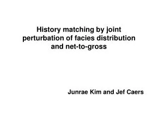
History matching by joint perturbation of facies distribution and net-to-gross. Junrae Kim and Jef Caers. Objectives. Constraining geological models to production data, adjusting aspects of geological model. Assessing value of information of production data on N/G.

E N D
History matching by joint perturbation of facies distribution and net-to-gross Junrae Kim and Jef Caers
Objectives • Constraining geological models to production data, adjusting aspects of geological model. • Assessing value of information of production data on N/G. • Application to a realistic 3D reservoir and well test.
P 50 Reference 50 I Motivation :N/G should not be fixed in history matching Flow response of 20 realizations N/G=0.05 N/G=0.6 • Elliptical bodies of high permeability • (1000 mD) in a lower permeability • matrix (15 mD) • Constant injection rate of 700 STB/day • No boundary conditions assumed • N/G (Reference) = 0.32
Jef Caers P(A|B) P(A|D) Model for P(A|B,D) Generate i(k+1)(u) rD = 1Full perturbation rD = 0No perturbation Probability perturbation method Perturb the conditional probabilities P(A|B) using another conditional probability that depends on the production data Define: P(A|D) = (1-rD) i(k)(u) + rD P(A) rD is found by solving a simple 1D optimization problem.
Couple perturbation of N/G with perturbation of rD. Perturbing N/G • Problem =>More difficult joint optimization of rD and N/G. • Solution =>Making proportional to rD : Back to 1D optimization • Why? =>High rD, : Big change in model
Couple perturbation of N/G with perturbation of rD. Increase Make linearly proportional to Decrease
Generate an initial guess realization Inner Loop Choose value for rD Choose value for rD Generate a new realization Outer Loop Calculate Calculate Define P(A|D) Generate a new realization & flow simulation Generate a new realization & flow simulation Change random seed No History match? Calculate O(-) Yes Calculate O(+) Run flow simulation Choose best rD and Obest from O(-) and O(+) Done Yes No Converged to best rD? The proposed method: basic algorithm Probability perturbation method: basic algorithm
P 50 Reference Conditioning data (facies) 50 I Training image 2-D reservoir model • Reference: 50 x 50 • Elliptical bodies of high permeability • (1000 mD) in a lower permeability • matrix (15 mD) • Constant injection rate of 700 STB/day • No boundary conditions assumed • N/G (Reference) = 0.32 • Training image: 150 x 150
Inner iteration Initial model Optimal value
Outer Iterations Reference Model
20 realizations 20 initial realizations 0.12 0.32 0.52 Initial N/G : Selected randomly from [0.12, 0.52] 20 history matched realizations Ref=0.32 Mean(H.M.)= 0.33 IQR=[0.28, 0.38]
20 realizations Initial N/G : Always 0.5 20 initial realizations 20 history matched realizations Ref=0.32 Mean(H.M.)= 0.33 IQR=[0.19, 0.45] Unbiased!!
Quantification of uncertainty on N/G from single well test • Investigate the value of information provided by a well test in a realistic 3D reservoir (Stanford V). • First: Spatial re-sampling to model the uncertainty on N/G without well test data: Journel (1993). • Second: Apply the proposed method. • 1. Use re-sampled N/G as initial guess • 2. History match • 3. Check final N/G from history matched realization
Quantification of uncertainty on N/G 3-D reservoir model • Dimensions 100x130x30 cells, three layers. • Fluvial channels (1500mD) in (50mD) permeability matrix. • Reference True N/G = 0.39. • A single vertical well (N/G = 0.5) available at x=52, y=65.
Quantification of uncertainty on N/G (First: without well test) What is the uncertainty without well test? => Spatial bootstrapping • Generate a geostatistical model conditioned to the single vertical well log data only; N/G realization = 0.5 • Randomly sample 20 vertical wells from the single geostatistical model. • Calculate N/G from 20 resampled wells. => N/G histogram
Quantification of uncertainty on N/G (Bootstrap) A spatial resampling of 20 wells N/G realization = 0.5 True Reference Training image True N/G = 0.4 Mean = 0.46 IQR = [0.33, 0.58] Wide confidence intervalUpward bias Resampled N/G
Quantification of uncertainty on N/G(Conditioning to well test data) What is the uncertainty with well test? • Each of the 20 re-sampled N/G is used as an initial guess. • 20 final history match generated • - perturbing facies and N/G. • Calculate N/G from final HM models. • => N/G Histogram
Quantification of uncertainty on N/G(Conditioning to well test data) Late Transient PSS/ Closed boundary Radial flow Well test model • A drawdown test for 100 days. • The rate of production is fixed to 1000 STB/day. • Boundary effect starts at 10 days.
Quantification of uncertainty on N/G(Conditioning to well test data) WBHP (initial guesses) WBHP (history matched)
Quantification of uncertainty on N/G(Conditioning to well test data) True N/G = 0.4 Original well log N/G = 0.5 Initial guesses (N/G) without well-test Mean = 0.46 IQR = [0.33, 0.58] History matched (N/G) with well-test Mean = 0.44 IQR = [0.40, 0.46] Reduction of uncertainty on N/G is significant.
Quantification of uncertainty on N/G(Conditioning to well test data) Pseudo steady state versus transient state 100 days 10 days 3 days • Variance in all cases are smaller than the case, where no well test is available. • The uncertainty is largest in the 3-day case. • Assumption: Averaging volume known (PSS)
Conclusions • N/G should not be fixed in a history matching process. • The proposed method jointly parameterizes perturbation of • N/G and of facies => simple & robust. • The method quantifies uncertainty of N/G based on • production data. • Well test: N/G can be quantified if averaging volume • is well known.
History matching by joint perturbation of P 50 50 I Facies anisotropy and facies distribution -90° 90° Case 2: Always starts from 0° Case 3 : Select randomly from [-90°, 90°] Case 1: Always starts from -45° Reference Mean: 47.6 [36, 58] Mean: 39.7 [30, 52] Mean: 44.0 [35, 52] IQR:
But still with large effort 45° 75° -15° -45° A history match was achieved in all cases…
3 days Reservoir N/G PSS The global N/G corresponding to the volume ratio Volume ratio corresponding to the number of days for which well test is run.