Download

1 / 32
320 likes | 347 Vues
Learn about experimental vs. non-experimental research, cross-sectional and longitudinal designs, multiple regression, and correlation studies in this comprehensive lecture. Explore the advantages and disadvantages of each approach.

E N D
URBDP 591 A Lecture 9: Cross-Sectional and Longitudinal Design Objectives • Experimental vs. Non-Experimental Design • Cross-Sectional Designs • Longitudinal Design • Multiple Regression
Experimental vs Correlational Research • experimental research determines whether one variable causes changes in another variable • correlational research measures the relationship between two variables • difference: variables can be related without being causally related
Correlational Research Main interest is to determine whether 2 variables co-vary and to determine direction of relationship. Characteristics of Correlational research. - Differs from experimental research: 1. No manipulation of IV's 2. Subjects not randomly assigned. - Measure 2 variables and determine whether correlational relationship exists between them. - If correlational relationship exists between 2 variables, can predict value of one variable from value of another
Correlational Studies • Type of descriptive research design • Advantage is that it can examine variables that cannot be experimentally manipulated (e.g.,population growth). • Disadvantage is that it cannot determine causality. • Third variable may account for the association. • Directionality unclear
Non-experimental Research Designs • Describes a particular situation or phenomenon. • Hypothesis generating • Can describe effect of implementing actions based on experimental research and help refine the implementation of these actions.
Cross-Sectional Study Designs • Compares groups at one point in time • e.g., landscape patterns. • Advantage is that it is an efficient way to identify possible group differences because you can study them at one point in time. • Disadvantage is that you cannot rule out cohort effects.
Non-Experimental Research Design • Longitudinal method--measurement of the same • subjects over time. • Cross-sectional method--measurement of several • groups at a single point in time. • Sequential methods--methods that combine the • cross-sectional and longitudinal methods
Longitudinal Design • Gathers data on a factor (e.g. bird diversity) over time. • Advantage is that you can see the time course of the development or change in the variables • Bird diversity decreasing with urbanization. • Bird diversity decreasing at a faster rate within the UGB. • Disadvantage is it is costly and still subject to bias
Cohort-Sequential Design • Combines a bit of the cross-sectional design and longitudinal design • E.g., Different bird species are compared on a variable over time. • Advantage – very efficient and reduces some of the biases in the cross-sectional design since you can see the evolution of change over time. • Disadvantage – cannot rule out cohort bias or the problem of the ‘unidentified’ third variable accounting for the change.
Correlational Research • correlation refers to a meaningful relationship between two variables; values of both variables change together somehow • positive correlation: high score on first variable associated with high score on second variable • negative correlation: high score on first variable associated with low score on second variable • no correlation: score on first variable not associated with score on second variable
Correlation vs. Regression Correlation Coefficient: Correlation tells us about the strength (and shape) of the relationship between two variables. The square of the correlation tells us the proportion of the variables' variance that is shared between them. Simple Regression: Regression tells us about the nature of the function relating the two variables. For linear regression, which is what we consider here, regression fits a straight line, called the regression line, to the data so that the line best describes their relationship. Multiple Regression Multiple regression tells us about the nature of the function that relates a set of predictor variables to a single response variable. OLS (ordinary least squares) multiple regression assumes the function is a linear function.
Covariance When there is a relation between two variables they covary. The Pearson correlation coefficient is a unit-free measure of the degree of covariance.
Covariance Now consider a third variable: A and B do not covary but C covary with both A and B None covary . They are orthogonal. A, B and C all covary The r2 is the amount of shared variation between the variables.
Measuring Correlations • scatterplots are used to provide a descriptive analysis of correlation – evaluate degree of relationship – assess linearity of relationship • Pearson’s r measures correlations between two interval/ratio level variables – magnitude measured from 0.0 to 1.0 – direction indicated by + or - – statistical significance of correlation provided by p value • Spearman’s rho measures correlations between two ordinal level variables
Interpreting Correlations • correlation is not causation • directionality problem • third-variable problem • partial correlation
Regression Analysis • regression allows prediction of a new observation based on what is known about correlation • regression involves drawing a line that best describes a correlation Y = a + bX + e • X is predictor variable; Y is criterion variable
The Multiple Regression Model A multiple regression equation expresses a linear relationship between a dependent variable Y and two or more independent variables (X1, X2, …, Xk) Y = α + β1X1 + β2X2 + … + βkXk + ε b is called a partial regression coefficient. For example, b1 denotes the coefficient of Y on variable X1 that one would expect if all the other X variables in the equation were held constant.
Meaning of parameter estimates • Slope • Change in Y per unit change in X. • Marginal contribution of X to Y holding all other variables in the regression constant. • Intercept • Meaningful only if X=0 is in the sample range. • Otherwise, merely extrapolation of linear approximation.
Coefficient of determination - R2 • Expresses the amount of variance on criterion explained by predictor or set of predictors • R2 increment - indicates the increase in the total variance on the criterion accounted for by each new predictor added to the regression model • 2 tests of significance are typically computed: i) is R different from 0, ii) is R2 increment statistically significant
Regression Equation for a Linear Relationship A linear relationship of n predictor variables, denoted X1, X2, ... Xn to a single response variable, denoted Y is described by the linear equation involving several variables. The general linear equation is: Y = a + b1X1 + b2X2 + ... + bnXn This equation shows that any linear relationship can be described by its: Intercept: The linear combination of the X's is zero. Slopes: The slope specifies how much the variable Y will change when the particular X changes by one unit.
Regression Assumptions 1. The independent variable should be accurately measured with negligible error. 2. The values of the dependent variable are normally distributed 3. Variation in the dependent variable (ie the spread around the line) is constant over values of the independent variable. This is known as homoscedasticity. 4. The values of residuals (the difference between the predicted and the expected values) have a normal distribution – that is, there are relatively few extremely small or extremely large residuals). 5. The values of the residuals are independent from each other – ie., they are randomly distributed along the regression line (there is no systematic pattern).
Multiregression problems • Outliers. As with SLR, a single outlying point can greatly distort the results of MLR, but it is more difficult to detect outliers visually. • Too few subject. A general rule of thumb is that you need at least 10-20 data points for each X variable, otherwise it is too easy to be misled with spurious results. • Inappropriate model. Although complicated, MLR is too simple for some data. MLR assumes that each X variable contributes independently towards the value of Y, but often X variables contribute to Y by an interaction with each other. • Unfocussed studies. If you give the computer enough variables, some significant relationships are bound to turn up by chance, and these may mean nothing.
Criteria for Developing a MLR Model • The overriding criterion is that any potential set of predictors must • be scientifically defensible. • It is not good science nor proper use of statistics to put predictors in • a model just because the data were available of to see “what happens”. • Other criteria: - A statistically significant overall model - A large R2. The model explains a large amount of variation in Y. • A small standard error (SQRT (MSE)) of the model. Is the • regression precise enough so that findings have practical utility? • Significant partial t tests. Does each X variable explain significant • additional variation in Y given the other predictors in the model? • Choose the smallest number of predictors to adequately • characterize the variation in Y.
Model Selection and Model Adequacy The model we can think of as having given rise to the observations is usually too complex to be described in every detail from the information available. We have to rely on more simple models; approximations Note: ”More realistic” models might be more close to ”the true model”. However, we are NOT aiming at finding the true model! We are trying to find THE BEST APPROXIMATING MODEL. The approximation should be sufficient for our purposes! Question: What’s sufficient?
How to select best model ”Best Model” Variance Bias Number of Parameters Trade-off between Bias and Variance when considering model complexity (number of parameters)
”delta” Model Selection: The Likelihood Ratio Test Basic idea: Add parameters only if they provide a significant improvement in the fit of the model to the data likelihood under Model 1 likelihood under Model 2
AIC = –2lnL +2N L= Likelihood N= Number of parameters Choose the model with the smallest AIC AIC penalizes the model for additional parameters Other alternatives for ranking models Akaike Information Criterion(AIC) An approximation of the Kullback–Liebler discrepancy
BIC = –2lnL + N ln n L= Likelihood N= Number of parameters n = number of characters Choose the model with the smallest BIC Other alternatives for ranking models Bayesian Information Criterion (BIC) An approximation of the log of the Bayes Factor For larger data, BIC should tend to choose simpler models than AIC (since the natural log of n is usually > 2)