Advanced GPS Surveying Techniques for Precise Navigation
120 likes | 239 Vues
Explore the modern technology of Global Positioning Systems (GPS) used for surveying, understanding the concept, measurements, sources of error, and differential correction to enhance accuracy in field surveys. Learn how to collect and store GPS data efficiently for mapping various geographic features.

Advanced GPS Surveying Techniques for Precise Navigation
E N D
Presentation Transcript
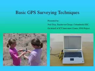
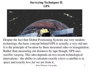
Surveying Techniques II.GPS Despite the fact that Global Positioning Systems use very modern technology, the basic concept behind GPS is actually a very old one: it is the principle of location by three measured sides or triangulation. Rather than measuring out distances by tape though, GPS uses satellite ranging. This idea depends on two recent technological innovations - the ability to calculate exactly where a satellite is in space and exactly how far we are from it. Harry Williams, Cartography
Triangulation is a little misleading however. There are 30 GPS satellites in orbit (as of May 24, 2010) and a GPS receiver usually uses 6 or 7 at a time to fix locations. Measuring distance from a satellite. How exactly do you measure accurately, distance between your location and a satellite? This is based on extremely accurate atomic clocks. GPS receivers and satellites both generate identical pseudo-random codes at precisely the same time. These codes are a series of radio signal pulses. The signal from a satellite can be received by a GPS receiver and then compared to its own internally generated code in order to calculate the time difference between them. This time difference is the time it took for the satellite signal to travel from the satellite to the receiver. Multiply this time difference by the speed of radio waves (186,000 miles per second) and you get your exact distance from the satellite. Harry Williams, Cartography
Receiver Satellite Time difference Harry Williams, Cartography
Sources of error in GPS measurements. There are several sources of error which can degrade GPS positional accuracy. Slight errors in satellite position, known as ephemeris errors, are caused by factors such as the gravitational pull of the moon. Another source of error is the earth's ionosphere - a band of electrically charged particles. This layer slows the GPS radio signal, giving the impression that the satellite is further away than it really is. Water vapor in the atmosphere can have the same effect as the ionosphere. Apart from ionospheric and atmospheric delay errors, small, but significant, clock and computational errors can also exist. There are also multipath errors - the signal from a satellite may "bounce around" before reaching the receiver. The angle between the receiver and satellite is another important consideration; the “Position Dilution of Precision" (PDOP) can magnify or lessen accuracy depending on these angles. Harry Williams, Cartography
Typical error amounts: Error Source Error Amount satellite clock error 0.75 m ephemeris error 0.75 m receiver error 1.50 m ionospheric/atmospheric 4.00 m The result of all sources of error and the Position Dilution Of Precision is a typical error of maybe 5-10 m under good conditions, maybe 50 m under poor conditions. Note: anything that can block radio signals (e.g. trees, buildings..) can degrade the GPS signal. Harry Williams, Cartography
Differential Correction. One of the ways of boosting GPS positional accuracy is based on another concept borrowed from traditional cartography - the use of a benchmark. The idea is to position a permanent GPS base station in a precisely known location. Using the resulting base files, the receiver files (or rover files) can be differentially corrected; this means that the offset due to error at the base station (which is found by comparing the base station's known position to its GPS-calculated position) can be applied to GPS positions collected in the field. After differential correction, a mapping-grade GPS receiver will give errors of maybe 1-2 m. Harry Williams, Cartography
Field Surveying with GPS. A GPS can map three kinds of geographic features – points, lines and polygons (areas). A convenient feature of a mapping-grade GPS is a data dictionary - a "shopping list" of the features and feature attributes you want to map for your project. You create the data dictionary prior to going into the field and download it to your GPS receiver. In the field, the data dictionary reminds you of what to record and the format of each record - as such it serves as a "protocol" for your project measurements (i.e. what is recorded and how it is recorded). The data dictionary is created and downloaded to the GPS via GPS software on a PC (e.g. PathFinder Office – a Trimble Navigation product). The data dictionary consists of features, attributes and a menu of possible choices… Harry Williams, Cartography
Storing Field Data:GPS data is collected in a rover file – a rover file is opened and named automatically as follows: File prefix (for example, C)Month (for example, 06 - June)Day (for example, 25)Hour (for example, 09*)A - the first file created in the 9th hour of June 25th. C062509A would be the file number (C062509B would be the 2nd file created in the same hour). *Coordinated Universal Time (UTC) system is based on Greenwich Mean Time (GMT). Opening a rover file usually brings up a list of options to select (e.g. select feature allows you to select (and begin mapping) features (e.g. tree, path, flower bed..). Harry Williams, Cartography
Mapping Point Features: Once the rover file is opened, features in the data dictionary can be selected to begin mapping (i.e. selecting a feature such as tree will cause the GPS to start recording positions). While positions are being recorded, the data dictionary can be used to select and enter attribute data (e.g. species of tree, height of tree, condition of tree, etc..). When you have collected enough positions for the point feature*, selecting close feature closes the feature and returns you to the select feature screen. You can then move to the next point to be mapped (e.g. another tree) and repeat the process. When all required features have been mapped, selecting close file closes the file. *how many positions do you collect? Positions are averaged to improve accuracy – a common value is 120 positions for one point feature. A common rate of recording positions for point features is 1 per second. Harry Williams, Cartography
Mapping Lines and Areas: This is similar to mapping points, except you have to walk or drive or fly etc. along the line or perimeter of the feature while collecting positions. The rate at which positions are recorded for line and area features can be selected within the GPS (usually 1 position every 5 seconds). If you are walking along a line feature, it is common to pause position recording so that attribute data can be entered using a data dictionary. We will use Trimble’s GeoXT – a hand-held mapping-grade GPS receiver. An online users guide is available here: http://www.docstoc.com/docs/672949/Trimble-GeoXT-Quick-Start-Guide Harry Williams, Cartography
Next week we cover: Differential correction Importing GPS data into a GIS Harry Williams, Cartography