Download
1 / 147
1.47k likes | 1.78k Vues
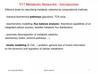
V17 Metabolic Networks - Introduction. Different levels for describing metabolic networks by computational methods: - classical biochemical pathways (glycolysis, TCA cycle, ... - stoichiometric modelling ( flux balance analysis ): theoretical capabilities of an

E N D
V17 Metabolic Networks - Introduction Different levels for describing metabolic networks by computational methods: - classical biochemical pathways (glycolysis, TCA cycle, ... - stoichiometric modelling (flux balance analysis): theoretical capabilities of an integrated cellular process, feasible metabolic flux distributions - automatic decomposition of metabolic networks (elementary nodes, extreme pathways ...) - kinetic modelling (E-Cell ...) problem: general lack of kinetic information on the dynamics and regulation of cellular metabolism Bioinformatics III
EcoCyc Database E.coli genome contains 4.7 million DNA bases. How can we characterize the functional complement of E.coli and according to what criteria can we compare the biochemical networks of two organisms? EcoCyc contains the metabolic map of E.coli defined as the set of all known pathways, reactions and enzymes of E.coli small-molecule metabolism. Analyze - the connectivity relationships of the metabolic network - its partitioning into pathways - enzyme activation and inhibition - repetition and multiplicity of elements such as enzymes, reactions, and substrates. Ouzonis, Karp, Genome Res. 10, 568 (2000) Bioinformatics III
EcoCyc Analysis of E.coli Metabolism E.coli genome contains 4391 predicted genes, of which 4288 code for proteins. 676 of these genes form 607 enzymes of E.coli small-molecule metabolism. Of those enzymes, 311 are protein complexes, 296 are monomers. Organization of protein complexes. Distribution of subunit counts for all EcoCyc protein complexes. The predominance of monomers, dimers, and tetramers is obvious Ouzonis, Karp, Genome Res. 10, 568 (2000) Bioinformatics III
Reactions EcoCyc describes 905 metabolic reactions that are catalyzed by E. coli. Of these reactions, 161 are not involved in small-molecule metabolism, e.g. they participate in macromolecule metabolism such as DNA replication and tRNA charging. Of the remaining 744 reactions, 569 have been assigned to at least one pathway. The next figures show an overview diagram of E. coli metabolism. Each node in the diagram represents a single metabolite whose chemical class is encoded by the shape of the node. Each blue line represents a single bioreaction. The white lines connect multiple occurrences of the same metabolite in the diagram. Ouzonis, Karp, Genome Res. 10, 568 (2000) Bioinformatics III
Reactions The number of reactions (744) and the number of enzymes (607) differ ... WHY?? (1) there is no one-to-one mapping between enzymes and reactions – some enzymes catalyze multiple reactions, and some reactions are catalyzed by multiple enzymes. (2) for some reactions known to be catalyzed by E.coli, the enzyme has not yet been identified. Ouzonis, Karp, Genome Res. 10, 568 (2000) Bioinformatics III
Compounds The 744 reactions of E.coli small-molecule metabolism involve a total of 791 different substrates. On average, each reaction contains 4.0 substrates. Number of reactions containing varying numbers of substrates (reactants plus products). Ouzonis, Karp, Genome Res. 10, 568 (2000) Bioinformatics III
Compounds Each distinct substrate occurs in an average of 2.1 reactions. Ouzonis, Karp, Genome Res. 10, 568 (2000) Bioinformatics III
Pathways EcoCyc describes 131 pathways: energy metabolism nucleotide and amino acid biosynthesis secondary metabolism Pathways vary in length from a single reaction step to 16 steps with an average of 5.4 steps. Length distribution of EcoCyc pathways Ouzonis, Karp, Genome Res. 10, 568 (2000) Bioinformatics III
Reactions Catalyzed by More Than one Enzyme Diagram showing the number of reactions that are catalyzed by one or more enzymes. Most reactions are catalyzed by one enzyme, some by two, and very few by more than two enzymes. For 84 reactions, the corresponding enzyme is not yet encoded in EcoCyc. What may be the reasons for isozyme redundancy? (1) the enzymes that catalyze the same reaction are homologs and have duplicated (or were obtained by horizontal gene transfer), acquiring some specificity but retaining the same mechanism (divergence) (2) the reaction is easily „invented“; therefore, there is more than one protein family that is independently able to perform the catalysis (convergence). Ouzonis, Karp, Genome Res. 10, 568 (2000) Bioinformatics III
Enzymes that catalyze more than one reaction Genome predictions usually assign a single enzymatic function. However, E.coli is known to contain many multifunctional enzymes. Of the 607 E.coli enzymes, 100 are multifunctional, either having the same active site and different substrate specificities or different active sites. Number of enzymes that catalyze one or more reactions. Most enzymes catalyze one reaction; some are multifunctional. The enzymes that catalyze 7 and 9 reactions are purine nucleoside phosphorylase and nucleoside diphosphate kinase. Take-home message: The high proportion of multifunctional enzymes implies that the genome projects significantly underpredict multifunctional enzymes! Ouzonis, Karp, Genome Res. 10, 568 (2000) Bioinformatics III
Reactions participating in more than one pathway The 99 reactions belonging to multiple pathways appear to be the intersection points in the complex network of chemical processes in the cell. E.g. the reaction present in 6 pathways corresponds to the reaction catalyzed by malate dehydrogenase, a central enzyme in cellular metabolism. Ouzonis, Karp, Genome Res. 10, 568 (2000) Bioinformatics III
Connectivity distributions P(k) for substrates a, Archaeoglobus fulgidus (archae); b, E. coli (bacterium); c, Caenorhabditis elegans (eukaryote), shown on a log–log plot, counting separately the incoming (In) and outgoing links (Out) for each substrate. kin (kout) corresponds to the number of reactions in which a substrate participates as a product (educt). d, The connectivity distribution averaged over 43 organisms. Jeong et al. Nature 407, 651 (2000) Bioinformatics III
Properties of metabolic networks a, The histogram of the biochemical pathway lengths, l, in E. coli. b, The average path length (diameter) for each of the 43 organisms. c, d, Average number of incoming links (c) or outgoing links (d) per node for each organism. e, The effect of substrate removal on the metabolic network diameter of E. coli. In the top curve (red) the most connected substrates are removed first. In the bottom curve (green) nodes are removed randomly. M = 60 corresponds to 8% of the total number of substrates in found in E. coli. The horizontal axis in b– d denotes the number of nodes in each organism. b–d, Archaea (magenta), bacteria (green) and eukaryotes (blue) are shown. The diameter of the network does not grow with N! Diameter of small world network grows with log N or even log log N! Jeong et al. Nature 407, 651 (2000) Bioinformatics III
Stoichiometric matrix Stoichiometric matrix: A matrix with reaction stochio-metries as columns and metabolite participations as rows. The stochiometric matrix is an important part of the in silico model. With the matrix, the methods of extreme pathway and elementary mode analyses can be used to generate a unique set of pathways P1, P2, and P3 (see future lecture). Papin et al. TIBS 28, 250 (2003) Bioinformatics III
Flux balancing Any chemical reaction requiresmass conservation. Therefore one may analyze metabolic systems by requiring mass conservation. Only required: knowledge about stoichiometry of metabolic pathways and metabolic demands For each metabolite: Under steady-state conditions, the mass balance constraints in a metabolic network can be represented mathematically by the matrix equation: S· v = 0 where the matrix S is the m n stoichiometric matrix, m = the number of metabolites and n = the number of reactions in the network. The vector v represents all fluxes in the metabolic network, including the internal fluxes, transport fluxes and the growth flux. Bioinformatics III
Flux balance analysis Since the number of metabolites is generally smaller than the number of reactions (m < n) the flux-balance equation is typically underdetermined. Therefore there are generally multiple feasible flux distributions that satisfy the mass balance constraints. The set of solutions are confined to the nullspace of matrix S. To find the „true“ biological flux in cells ( e.g. Heinzle, Huber, UdS) one needs additional (experimental) information, or one may impose constraints on the magnitude of each individual metabolic flux. The intersection of the nullspace and the region defined by those linear inequalities defines a region in flux space = the feasible set of fluxes. Bioinformatics III
Feasible solution set for a metabolic reaction network (A) The steady-state operation of the metabolic network is restricted to the region within a cone, defined as the feasible set. The feasible set contains all flux vectors that satisfy the physicochemical constrains. Thus, the feasible set defines the capabilities of the metabolic network. All feasible metabolic flux distributions lie within the feasible set, and (B) in the limiting case, where all constraints on the metabolic network are known, such as the enzyme kinetics and gene regulation, the feasible set may be reduced to a single point. This single point must lie within the feasible set. Edwards & Palsson PNAS 97, 5528 (2000) Bioinformatics III
Summary FBA analysis constructs the optimal network utilization simply using stoichiometry of metabolic reactions and capacity constraints. For E.coli the in silico results are consistent with experimental data. FBA shows that in the E.coli metabolic network there are relatively few critical gene products in central metabolism. However, the the ability to adjust to different environments (growth conditions) may be dimished by gene deletions. FBA identifies „the best“ the cell can do, not how the cell actually behaves under a given set of conditions. Here, survival was equated with growth. FBA does not directly consider regulation or regulatory constraints on the metabolic network. This can be treated separately (see future lecture). Edwards & Palsson PNAS 97, 5528 (2000) Bioinformatics III
V18 – extreme pathways • Computational metabolomics: modelling constraints • Surviving (expressed) phenotypes must satisfy constraints imposed on the molecular functions of a cell, e.g. conservation of mass and energy. • Fundamental approach to understand biological systems: identify and formulate constraints. • Important constraints of cellular function: • physico-chemical constraints • Topological constraints • Environmental constraints • Regulatory constraints Price et al. Nature Rev Microbiol 2, 886 (2004) Bioinformatics III
Physico-chemical constraints These are „hard“ constraints: Conservation of mass, energy and momentum. Contents of a cell are densely packed viscosity can be 100 – 1000 times higher than that of water Therefore, diffusion rates of macromolecules in cells are slower than in water. Many molecules are confined inside the semi-permeable membrane high osmolarity. Need to deal with osmotic pressure (e.g. Na+K+ pumps) Reaction rates are determined by local concentrations inside cells Enzyme-turnover numbers are generally less than 104 s-1. Maximal rates are equal to the turnover-number multiplied by the enzyme concentration. Biochemical reactions are driven by negative free-energy change in forward direction. Price et al. Nature Rev Microbiol 2, 886 (2004) Bioinformatics III
Topological constraints The crowding of molecules inside cells leads to topological (3D)-constraints that affect both the form and the function of biological systems. E.g. the ratio between the number of tRNAs and the number of ribosomes in an E.coli cell is about 10. Because there are 43 different types of tRNA, there is less than one full set of tRNAs per ribosome it may be necessary to configure the genome so that rare codons are located close together. E.g. at a pH of 7.6 E.coli typically contains only about 16 H+ ions. Remember that H+ is involved in many metabolic reactions. Therefore, during each such reaction, the pH of the cell changes! Price et al. Nature Rev Microbiol 2, 886 (2004) Bioinformatics III
Environmental constraints Environmental constraints on cells are time and condition dependent: Nutrient availability, pH, temperature, osmolarity, availability of electron acceptors. E.g. Heliobacter pylori lives in the human stomach at pH = 1 needs to produce NH3 at a rate that will maintain ist immediate surrounding at a pH that is sufficiently high to allow survival. Ammonia is made from elementary nitrogen H. pylori has adapted by using amino acids instead of carbohydrates as its primary carbon source. Price et al. Nature Rev Microbiol 2, 886 (2004) Bioinformatics III
Regulatory constraints Regulatory constraints are self-imposed by the organism and are subject to evolutionary change they are no „hard“ constraints. Regulatory constraints allow the cell to eliminate suboptimal phenotypic states and to confine itself to behaviors of increased fitness. Q: classify the following constrains as physico-chemical, regulatory and topological restraints ... Multiple-choice selection. Price et al. Nature Rev Microbiol 2, 886 (2004) Bioinformatics III
Mathematical formation of constraints There are two fundamental types of constraints: balances and bounds. Balances are constraints that are associated with conserved quantities as energy, mass, redox potential, momentum or with phenomena such as solvent capacity, electroneutrality and osmotic pressure. Bounds are constraints that limit numerical ranges of individual variables and parameters such as concentrations, fluxes or kinetic constants. Both bound and balance constraints limit the allowable functional states of reconstructed cellular metabolic networks. Price et al. Nature Rev Microbiol 2, 886 (2004) Bioinformatics III
Extreme Pathways introduced into metabolic analysis by the lab of Bernard Palsson (Dept. of Bioengineering, UC San Diego). The publications of this lab are available at http://gcrg.ucsd.edu/publications/index.html The extreme pathway technique is based on the stoichiometric matrix representation of metabolic networks. All external fluxes are defined as pointing outwards. Schilling, Letscher, Palsson, J. theor. Biol. 203, 229 (2000) Bioinformatics III
Extreme Pathways – theorem Theorem. A convex flux cone has a set of systemically independent generating vectors. Furthermore, these generating vectors (extremal rays) are unique up to a multiplication by a positive scalar. These generating vectors will be called „extreme pathways“. Proof. omitted. Bioinformatics III
Extreme Pathways – algorithm - setup The algorithm to determine the set of extreme pathways for a reaction network follows the pinciples of algorithms for finding the extremal rays/ generating vectors of convex polyhedral cones. Combine n n identity matrix (I) with the transpose of the stoichiometric matrix ST. I serves for bookkeeping. Schilling, Letscher, Palsson, J. theor. Biol. 203, 229 (2000) S I ST Bioinformatics III
separate internal and external fluxes Examine constraints on each of the exchange fluxes as given by j bj j If the exchange flux is constrained to be positive do nothing. If the exchange flux is constrained to be negative multiply the corresponding row of the initial matrix by -1. If the exchange flux is unconstrained move the entire row to a temporary matrix T(E). This completes the first tableau T(0). T(0) and T(E) for the example reaction system are shown on the previous slide. Each element of this matrices will be designated Tij. Starting with x = 1 and T(0) = T(x-1) the next tableau is generated in the following way: Schilling, Letscher, Palsson, J. theor. Biol. 203, 229 (2000) Bioinformatics III
idea of algorithm (1) Identify all metabolites that do not have an unconstrained exchange flux associated with them. The total number of such metabolites is denoted by . For the example, this is only the case for metabolite C ( = 1). What is the main idea? - We want to find balanced extreme pathways that don‘t change the concentrations of metabolites when flux flows through (input fluxes are channelled to products not to accumulation of intermediates). - The stochiometrix matrix describes the coupling of each reaction to the concentration of metabolites X. - Now we need to balance combinations of reactions that leave concentrations unchanged. Pathways applied to metabolites should not change their concentrations the matrix entries need to be brought to 0. Schilling, Letscher, Palsson, J. theor. Biol. 203, 229 (2000) Bioinformatics III
keep pathways that do not change concentrations of internal metabolites (2) Begin forming the new matrix T(x) by copying all rows from T(x – 1) which contain a zero in the column of ST that corresponds to the first metabolite identified in step 1, denoted by index c. (Here 3rd column of ST.) Schilling, Letscher, Palsson, J. theor. Biol. 203, 229 (2000) T(0) = T(1) = + Bioinformatics III
balance combinations of other pathways (3) Of the remaining rows in T(x-1) add together all possible combinations of rows which contain values of the opposite sign in column c, such that the addition produces a zero in this column. Schilling, et al. JTB 203, 229 T(0) = T(1) = Bioinformatics III
remove “non-orthogonal” pathways (4) For all of the rows added to T(x) in steps 2 and 3 check to make sure that no row exists that is a non-negative combination of any other sets of rows in T(x) . One method used is as follows: let A(i) = set of column indices j for with the elements of row i = 0. For the example above Then check to determine if there exists A(1) = {2,3,4,5,6,9,10,11} another row (h) for which A(i) is a A(2) = {1,4,5,6,7,8,9,10,11} subset of A(h). A(3) = {1,3,5,6,7,9,11} A(4) = {1,3,4,5,7,9,10} If A(i) A(h),i h A(5) = {1,2,3,6,7,8,9,10,11} where A(6) = {1,2,3,4,7,8,9} A(i) = { j : Ti,j = 0, 1 j (n+m) } then row i must be eliminated from T(x) Schilling et al. JTB 203, 229 Bioinformatics III
repeat steps for all internal metabolites (5) With the formation of T(x) complete steps 2 – 4 for all of the metabolites that do not have an unconstrained exchange flux operating on the metabolite, incrementing x by one up to . The final tableau will be T(). Note that the number of rows in T () will be equal to k, the number of extreme pathways. Schilling et al. JTB 203, 229 Bioinformatics III
balance external fluxes (6) Next we append T(E) to the bottom of T(). (In the example here = 1.) This results in the following tableau: Schilling et al. JTB 203, 229 T(1/E) = Bioinformatics III
balance external fluxes (7) Starting in the n+1 column (or the first non-zero column on the right side), if Ti,(n+1) 0 then add the corresponding non-zero row from T(E) to row i so as to produce 0 in the n+1-th column. This is done by simply multiplying the corresponding row in T(E) by Ti,(n+1) and adding this row to row i . Repeat this procedure for each of the rows in the upper portion of the tableau so as to create zeros in the entire upper portion of the (n+1) column. When finished, remove the row in T(E) corresponding to the exchange flux for the metabolite just balanced. Schilling et al. JTB 203, 229 Bioinformatics III
balance external fluxes (8) Follow the same procedure as in step (7) for each of the columns on the right side of the tableau containing non-zero entries. (In this example we need to perform step (7) for every column except the middle column of the right side which correponds to metabolite C.) The final tableau T(final) will contain the transpose of the matrix P containing the extreme pathways in place of the original identity matrix. Schilling et al. JTB 203, 229 Bioinformatics III
pathway matrix T(final) = PT = Schilling et al. JTB 203, 229 v1 v2 v3 v4 v5 v6 b1 b2 b3 b4 p1 p7 p3 p2 p4 p6 p5 Bioinformatics III
Extreme Pathways for model system 2 pathways p6 and p7 are not shown (right below) because all exchange fluxes with the exterior are 0. Such pathways have no net overall effect on the functional capabilities of the network. They belong to the cycling of reactions v4/v5 and v2/v3. Schilling et al. JTB 203, 229 v1 v2 v3 v4 v5 v6 b1 b2 b3 b4 p1 p7 p3 p2 p4 p6 p5 Bioinformatics III
How reactions appear in pathway matrix In the matrix P of extreme pathways, each column is an EP and each row corresponds to a reaction in the network. The numerical value of the i,j-th element corresponds to the relative flux level through the i-th reaction in the j-th EP. Papin, Price, Palsson, Genome Res. 12, 1889 (2002) Bioinformatics III
Properties of pathway matrix A symmetric Pathway Length Matrix PLM can be calculated: where the values along the diagonal correspond to the length of the EPs. The off-diagonal terms of PLM are the number of reactions that a pair of extreme pathways have in common. Papin, Price, Palsson, Genome Res. 12, 1889 (2002) Bioinformatics III
Properties of pathway matrix One can also compute a reaction participation matrix PPM from P: where the diagonal correspond to the number of pathways in which the given reaction participates. Papin, Price, Palsson, Genome Res. 12, 1889 (2002) Bioinformatics III
Application of elementary modesMetabolic network structure of E.coli determineskey aspects of functionality and regulation Elementary modes will be covered in V19. The concept is closely related to extreme pathways. In this example , we will simply ignore the small difference. Compute EFMs for central metabolism of E.coli. Catabolic part: substrate uptake reactions, glycolysis, pentose phosphate pathway, TCA cycle, excretion of by-products (acetate, formate, lactate, ethanol) Anabolic part: conversions of precursors into building blocks like amino acids, to macromolecules, and to biomass. Stelling et al. Nature 420, 190 (2002) Bioinformatics III
Metabolic network topology and phenotype The total number of EFMs for given conditions is used as quantitative measure of metabolic flexibility. a, Relative number of EFMs N enabling deletion mutants in gene i (i) of E. coli to grow (abbreviated by µ) for 90 different combinations of mutation and carbon source. The solid line separates experimentally determined mutant phenotypes, namely inviability (1–40) from viability (41–90). Stelling et al. Nature 420, 190 (2002) The # of EFMs for mutant strain allows correct prediction of growth phenotype in more than 90% of the cases. Bioinformatics III
Robustness analysis The # of EFMs qualitatively indicates whether a mutant is viable or not, but does not describe quantitatively how well a mutant grows. Define maximal biomass yield Ymass as the optimum of: eiis the single reaction rate (growth and substrate uptake) in EFM i selected for utilization of substrate Sk. Stelling et al. Nature 420, 190 (2002) Bioinformatics III
Can regulation be predicted by EFM analysis? Compute control-effective fluxes for each reaction l by determining the efficiency of any EFM eiby relating the system‘s output to the substrate uptake and to the sum of all absolute fluxes. With flux modes normalized to the total substrate uptake, efficiencies i(Sk, ) for the targets for optimization -growth and ATP generation, are defined as: Control-effective fluxes vl(Sk) are obtained by averaged weighting of the product of reaction-specific fluxes and mode-specific efficiencies over all EFMs using the substrate under consideration: YmaxX/Si and YmaxA/Si are optimal yields of biomass production and of ATP synthesis. Control-effective fluxes represent the importance of each reaction for efficient and flexible operation of the entire network. Stelling et al. Nature 420, 190 (2002) Bioinformatics III
Prediction of gene expression patterns As cellular control on longer timescales is predominantly achieved by genetic regulation, the control-effective fluxes should correlate with messenger RNA levels. Compute theoretical transcript ratios (S1,S2) for growth on two alternative substrates S1 and S2 as ratios of control-effective fluxes. Compare to exp. DNA-microarray data for E.coli growin on glucose, glycerol, and acetate. Excellent correlation! Stelling et al. Nature 420, 190 (2002) Calculated ratios between gene expression levels during exponential growth on acetate and exponential growth on glucose (filled circles indicate outliers) based on all elementary modes versus experimentally determined transcript ratios19. Lines indicate 95% confidence intervals for experimental data (horizontal lines), linear regression (solid line), perfect match (dashed line) and two-fold deviation (dotted line). Bioinformatics III
Summary (extreme pathways) Extreme pathway analysis provides a mathematically rigorous way to dissect complex biochemical networks. The matrix products PT P and PT P are useful ways to interpret pathway lengths and reaction participation. However, the number of computed vectors may range in the 1000sands. Therefore, meta-methods (e.g. singular value decomposition) are required that reduce the dimensionality to a useful number that can be inspected by humans. Single value decomposition may be one useful method ... and there are more to come. Price et al. Biophys J 84, 794 (2003) Bioinformatics III
V19 Metabolic Pathway Analysis (MPA) Metabolic Pathway Analysis searches for meaningful structural and functional units in metabolic networks. Today‘s most powerful methods are based on convex analysis. Two such approaches are the elementary flux modes (Schuster et al. 1999, 2000) and extreme pathways (Schilling et al. 2000). Both sets span the space of feasible steady-state flux distributions by non-decomposable routes, i.e. no subset of reactions involved in an EFM or EP can hold the network balanced using non-trivial fluxes. MPA can be used to study e.g. - routing + flexibility/redundancy of networks - functionality of networks - idenfication of futile cycles - gives all (sub)optimal pathways with respect to product/biomass yield - can be useful for calculability studies in MFA Klamt et al. Bioinformatics 19, 261 (2003) Bioinformatics III
Metabolic Pathway Analysis: Elementary Flux Modes The technique of Elementary Flux Modes (EFM) was developed prior to extreme pathways (EP) by Stephan Schuster, Thomas Dandekar and co-workers: Pfeiffer et al. Bioinformatics, 15, 251 (1999) Schuster et al. Nature Biotech. 18, 326 (2000) The method is very similar to the „extreme pathway“ method to construct a basis for metabolic flux states based on methods from convex algebra. Extreme pathways are a subset of elementary modes, and for many systems, both methods coincide. Are the subtle differences important? Bioinformatics III
Elementary Flux Modes Start from list of reaction equations and a declaration of reversible and irreversible reactions and of internal and external metabolites. E.g. reaction scheme of monosaccharide Fig.1 metabolism. It includes 15 internal metabolites, and 19 reactions. S has dimension 15 19. It is convenient to reduce this matrix by lumping those reactions that necessarily operate together. {Gap,Pgk,Gpm,Eno,Pyk}, {Zwf,Pgl,Gnd} Such groups of enzymes can be detected automatically. This reveals another two sequences {Fba,TpiA} and {2 Rpe,TktI,Tal,TktII}. Schuster et al. Nature Biotech 18, 326 (2000) Bioinformatics III