Structural analysis of metabolic networks
320 likes | 547 Vues
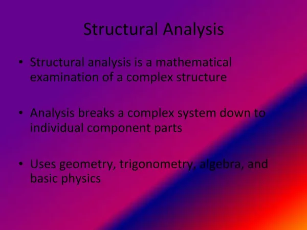
Structural analysis of metabolic networks. Ms. Shivani Bhagwat Lecturer, School of Biotechnology DAVV. Structural analysis of metabolic networks Global network properties Knowledge about the topological properties of a metabolic network(MN) is central to the understanding of its function.

Structural analysis of metabolic networks
E N D
Presentation Transcript
Structuralanalysis of metabolic networks Ms. Shivani Bhagwat Lecturer, School of Biotechnology DAVV
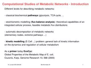
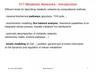
Structural analysis of metabolic networks Global network properties Knowledge about the topological properties of a metabolic network(MN) is central to the understanding of its function. Graph theoretic approaches have been extensively employed to derive global network features such as topological organization and robustness properties (Ravasz, 2003 and Palsson, 2006), determine the importance of individual enzymes or metabolites and curate the network by predicting missing components. A number of graph theoretic measures describe the global structure of MNs (Discrete Models and Mathematics, Graph Theoretic Approaches). The degree distribution is the probability distribution of links per node (degree) in a network. A small number of metabolites act as hubs involved in a very large number of reactions (e.g. ATP, Coenzyme A), making the network extremely robust to random loss of nodes.
Discrete Models and Mathematics: Discrete mathematics is the study of mathematical structures that are fundamentally discrete rather than continuous. Graph Theoretic Approaches: For many species, multiple maps are available, often constructed independently by different research groups using different sets of markers and different source material. Integration of these maps provides a higher density of markers and greater genome coverage than is possible using a single study.
Local network analysis In addition to local versions of the measures, attempts have been made to examine the network on a local scale. Network motifs, defined as sub-networks that occur significantly more often in a network than expected by chance, have been identified and shown to perform specific tasks in MNs. Among them are futile cycles that dissipate energy in the MN, switches directing the metabolite flux and feed-forward motifs that provide regulatory control. Overall, it appears that the recurrence of such local architecture enables biological adaptation to varying environments. The number of shared neighbors between two nodes is called a topological overlap. By calculating it for every node and subsequent clustering (Clustering), a topological overlap map can be generated. Metabolites with similar biochemical properties cluster together, demonstrating functional organization of sub networks in MNs.
From static to dynamic models Despite their usefulness, graph-based approaches do not depict the dynamical behavior of metabolic networks. However, stoichiometry based approaches and kinetic models permit to investigate the fluxes of metabolites within metabolic pathways, which is of great interest with respect to functional analysis of metabolism and pharmacological studies. Boolean network analysis (BNA) use Boolean logic to infer the capacity to produce given metabolites and the activities of given reactions, by treating each node as a switch that can either be on or off. After setting appropriate starting states, in which certain reactions are switched off, the state of all other nodes is determined by iteratively applying Boolean rules, until no further change occurs. BNA has been applied successfully in model curation and network robustness analysis.
Network expansion is a method closely related to BNA: Starting with a seed of nutrients, the so called scope (all producible metabolites and active reactions) is determined iteratively, based on Boolean state switches. Thus, the biosynthetic capacities of a MN can be assessed. Petri nets are directed bipartite graphs that are capable of modelling a discrete flow of mass within a MN. They are supported by a well--‐developed mathematical theory that even allows a transition to continuous simulations. Chemical reaction network theory (CRNT) and species reaction graphs (SR graphs) use topology and a few basic assumptions to derive the stability (Stability) and the possibility of multistability (Bistability) of a MN. However, due to their computational complexity, they are unsuitable at present for genome scale models. metabolic network dynamics are dependent on a multitude of factors in addition to network structure: reaction thermodynamics, kinetics and rates environmental conditions
Flux balance analysis (FBA) calculates optimal reaction rates at steady state in the network (flux distribution) by formulating a linear optimization problem. Reaction rates are constrained by the network stoichiometry, metabolite availability and thermodynamic properties of the catalysing enzymes. FBA is especially useful for simulating network disturbances, such as enzyme loss or nutrient shortage.
STOICHIOMETRY OF CELLULAR REACTIONS The overall result of the totality of cellular reactions is the conversion of substrates into free energy and metabolic products (e.g., primary metabolites),more complex products (such as secondary metabolites), extracellular proteins and constituents of biomass, e.g., cellular proteins, RNA, DNA, and lipids. These conversions occur via a large number of metabolites, including precursor metabolites and building blocks in the synthesis of macromolecular pools. In cellular reactions there are a number of cofactor pairs, with ATP/ADP, NAD+/NADH, and NADP+/NADPH being the most important. For the two compounds in a cofactor pair, the stoichiometric coefficients will normally be the same in magnitude but of opposite sign, e.g. the stoichiometric coefficients for NADPH and NADP+ are -1 and 1 respectively.
Example: Mixed Acid Fermentation by E. coli • E. coli is a facultative anaerobe that mediates a relatively complex fermentation normally referred to as mixed acid fermentation. • Seven metabolic products are produced, and with the exception of succinate, which is made from phosphoenolpyruvate, all metabolites are formed from pyruvate. • Succinate is formed via oxaloacetate, which undergoes transamination with glutamate to yield aspartate (one NADPH and one ammonium are used to regenerate glutamate from a-ketoglutarate, so they appear as reactants. • Aspartate is then deaminated to form fumarate, which is finally reduced to succinate by fumarate dehydrogenase (which is different from the succinate dehydrogenase that functions in the opposite direction). • Our goal in setting up a stoichiometric model is to account for the n e t change of metabolites in the medium in the context of catabolic reactions operative in a typical E. coli cell.
The conversion of glucose to phosphoenolpyruvate (PEP) is lumped into an overall reaction with the following stoichiometry : 8 overall reactions 1/2glucose + PEP + NADH= 0 -PEP - CO 2 - 2NADH + succinate = 0 -PEP + pyruvate + ATP = 0 -pyruvate- NADH + lactate = 0 -pyruvate + acetyl-CoA + formate = 0 -formate + CO 2 + H2 = 0 -acetyl-CoA + acetate + ATP = 0 -acetyl-CoA- 2NADH + ethanol = 0 Glucose is identified as a substrate and succinate, carbon dioxide, lactate, formate, hydrogen, acetate, and ethanol as metabolic products, with phosphenolpyruvate (PEP), pyruvate, acetyl-CoA, ATP, and NADH as intracellular metabolites.
ATP is produced only in two reactions, namely, the conversion of PEP to pyruvate and the conversion of acetyl-CoA to acetate. Because the fluxes of these two reactions are measurable (the flux to acetate can be measured directly as the formation rate of acetate, whereas the flux from PEP to pyruvate can be measured from the sum of the rates of formation of all the metabolic products except succinate or from the difference between the glucose uptake rate and the rate of succinate formation), we can obtain information on the total rate of ATP synthesis. As there are no other sources of ATP supply under anaerobic conditions, the latter is also an estimate of the consumption rate of ATP for growth and maintenance.
DYNAMIC MASS BALANCES A mass balance (also called a material balance) is an application of conservation of mass to the analysis of physical systems. By accounting for material entering and leaving a system, mass flows can be identified which might have been unknown, or difficult to measure. Input = output + accumulation Dynamics of the bioreactor Batch: where F - Fout = 0, i.e., the volume is constant. Batch experiments have the advantage of being easy to perform and can produce large volumes of experimental data in a short period of time. The disadvantage is that the experimental data are difficult to interpret as there are dynamic variations throughout the experiment, i.e., the environmental conditions experienced by the cells vary with time. By using well-instrumented bioreactors at least some variables, e.g., pH and dissolved oxygen tension, may, however, be controlled at a constant level.
Continuous: where F = F out ≠ 0 , i.e., the volume is constant. A typical operation of the continuous bioreactor is the so-called chemostat, where the added medium is designed such that there is a single rate-limiting substrate. This allows for controlled variation in the specific growth rate of the biomass. The advantage of the continuous bioreactor is that a steady state can be obtained, which allows for precise experimental determination of specific rates under well-defined environmental conditions. The disadvantage of the continuous bioreactor is that it is laborious to operate as large amounts of fresh, sterile medium have to be prepared and requires long periods of time for a steady state to be achieved. Fed-batch (or semibatch): where F ≠ 0 and F out = 0, i.e., the volume increases. This is probably the most common operation in industrial practice, because it allows for control of the environmental conditions, e.g., maintaining the glucose concentration at a certain level, and it enables formation of much higher titers Dynamic mass balances for the substrate will be : Substrate = - rate of substrate consumption + rate of substrate addition – rate of accumulation substrate removal
The specific substrate consumption rate of the ith substrate, x is the biomass concentration (g DW L -1) D is the so-called dilution rate (h -1) Which is zerofor a batch reactor and for a chemostat and a fed-batch reactor is given by: D= F/V rate of substrate consumption = specific rate of substrate consumption X biomass concentration. At steady state the accumulation term is equal to zero, so that the volumetric rate of substrate consumption becomes equal to the product of the dilution rate multiplied by the difference in the substrate concentrations between the inlet and outlet of the reactor. Another approach is to carry out a functional representation of the data,e.g., polynomial splining, and to calculate the derivatives and specific rates from the fitted functions. This approach too can give rise to large fluctuations in the specific rates, because it is difficult to find good functional representations of experimental cultivation data.
YIELD COEFFICIENTS AND LINEAR RATE EQUATIONS Macroscopic assessment of the overall distribution of metabolic fluxes, e.g., how much carbon in the glucose substrate is recovered in the metabolite of interest. This overall distribution of fluxes is normally represented by the so-called yield coefficients. Yield coefficients are, therefore, dimensionless and take the form of unit mass of metabolite per unit mass of the reference, e.g., moles of lysine produced per moles of glucose consumed. The moles of carbon dioxide produced per mole of oxygen consumed, called the respiratory quotient (RQ), frequently is used to characterize aerobic cultivations.
Metabolic Model of Penicillium chrysogenum we consider a simple metabolic model for the filamentous fungus P. chrysogenum as presented by Nielsen (1997). The stoichiometric model summarizes the overall cellular metabolism, and by employing pseudo-steady state assumptions for ATP, NADH, and NADPH metabolites, it is possible to derive linear rate equations where the specific uptake rates for glucose and oxygen and the specific carbon dioxide formation rate are expressed in terms of the specific growth rate. By evaluating the parameters in these linear rate expressions, which can be done from a comparison with experimental data, information on key energetic parameters may be extracted. In the analysis, formation of metabolites (both primary metabolites like gluconate and metabolites related to penicillin biosynthesis) was neglected, because the carbon flux to these products was small compared with the flux to biomass and carbon dioxide. The overall stoichiometry for synthesis of the constituents of a P. chrysogenum cell can be summarized as (Nielsen, 1997): Biomass + 0.139CO 2 + 0.458NADH- 1.139CH20- 0.20NH3 - 0.004 H2SO4- 0-010 H3PO4 - Y xATP ATP - 0.243NADPH = 0
Material Balances and Data Consistency Quantitative analysis of metabolism requires experimental data for the determination of metabolic fluxes, flux distributions, and measures of flux Control. In the context of metabolic analysis, flux calculations are based on the measurement of the specific rates for substrate uptake and product formation, which represent the fluxes in and out of the cells. Data redundancy is introduced when multiple sensors are employed for the measurement of the same variable or when certain constraints must be satisfied by the measurements so obtained, such as closure of material balances. Obviously, the greater the redundancy, the higher the degree of confidence for the data and their derivative parameters.
Experimental data that are to be used for quantitative analysis must be: • Complete • Noise free • There are two approaches in assessing the consistency of experimental data. • The first is based on a very simple metabolic model, the so-called black box • model, where all cellular reactions are lumped into a single one for the • overall cell biomass growth, and the method basically consists of validating • elemental balances. • The second approach recognizes far more biochemical detail in the overall conversion of substrates into biomass and metabolic products. As such, it is mathematically more involved, but, of course, it provides a more realistic depiction of the actual degrees of freedom than a black box model.
THE BLACK BOX MODEL Cell biomass is the black box exchanging material with the environment, and processing it through many cellular reactions lumped into one, that of biomass growth. The fluxes in and out of the black box are given by the specific rates (in grams or moles of the compound per gram or mole of biomass and unit time). These are the specific substrate uptake rates and the specific product formation rates. Representation of the black box model. The cell is considered as a black box, and fluxes in and out of the cell are the only variables measured. The fluxes of substrates into the cell are elements of the vector r s, and the fluxes of metabolic products out of the cell are elements of the vector r p. Some of the mass originally present in the substrates accumulates within the black box as formation of new biomass with the specific rate µ.
Use of the black box model for analyzing data consistency, one may use either: (1) A set of yield coefficients together with the specific growth rate (2) a set of yield coefficients with respect to another reference, e.g., one of the substrates, along with the specific rate of formation/consumption of reference compound (3) a set of specific rates for all substrates and products, including biomass 4) a set of all volumetric rates that are the product of the specific rates by the biomass concentration.
Black Box Model example: Consider the aerobic cultivation of the yeast Saccharomyces cerevisiae on a defined, minimal medium, i.e., glucose is the carbon and energy source and ammonia is the nitrogen source. During aerobic growth, the yeast oxidizes glucose completely to carbon dioxide. However, at very high glycolytic fluxes, a bottleneck in the oxidation of pyruvate leads to ethanol formation. Thus, at high glycolytic fluxes, both ethanol and carbon dioxide should be considered as metabolic products. Finally, water is formed in the cellular pathways, and this is also included as a product in the overall reaction. The stoichiometric (or yield) coefficients are not constant, as yield is zero at low specific growth rates (corresponding to low glycolytic fluxes) and greater than zero for higher specific growth rates.
ELEMENTAL BALANCES In the black box model, we have M + N + 1 variables: M yield coefficients for the metabolic products, N yield coefficients for the substrates, the forward reaction rate µ or the M + N + 1 specific rates . Because mass is conserved in the overall conversion of substrates to metabolic products and biomass, the (M + N + 1) rates of the black box model are not completely independent but must satisfy several constraints. Thus, the elements flowing into the system must balance the elements flowing out of the system, e.g., the carbon entering the system via the substrates has to be recovered in the metabolic products and biomass. Each element considered in the black box obviously yields one constraint.
HEAT BALANCE In the conversion of substrates to metabolic products and biomass, part of the Gibbs free energy in the substrates is dissipated to the surrounding environment as heat. Especially under aerobic conditions, the energy dissipation may be substantial. Energy dissipation is determined by the difference between the total Gibbs free energy in the substrates and the total Gibbs free energy recovered in the metabolic products and biomass. The energy dissipation normally gives rise to changes in both the enthalpy and entropy of the system, and it is difficult to quantify. Attention is, therefore, generally focused on heat production determined by the change in enthalpy, as this heat production has direct consequences for process cooling requirements for temperature control.
Metabolic flux analysis(MFA) • The first step in the process is to identify a desired goal to achieve through the improvement or modification of an organism's metabolism or, • Step I: system definition • Step II: mass balance • Step III: defining measurable fluxes • Step IV: optimization • The databases contain genomic and chemical information including pathways for metabolism and other cellular processes. From this an organism is chosen that will be used to create the desired product or result. • Considerations that are taken into account are: • how close the organism's metabolic pathway is to the desired pathway • the maintenance costs associated with the organism • how easy it is to modify the pathway of the organism. • Escherichia coli (E. coli) is widely used in metabolic engineering to synthesize a wide variety of products such as amino acids because it is relatively easy to maintain and modify. If the organism does not contain the complete pathway for the desired product or result, then genes that produce the missing enzymes must be incorporated into the organism
Analyzing a metabolic pathway The completed metabolic pathway is modeled mathematically to find the theoretical yield of the product or the reaction fluxes in the cell. A flux is the rate at which a given reaction in the network occurs. Simple metabolic pathway analysis can be done by hand, but most require the use of software to perform the computations. These programs use complex linear algebra algorithms to solve these models. To solve a network using the equation for determined systems . Information about the reaction (such as the reactants and stoichiometry) are contained in the matrices Gx and Gm. Matrices Vm and Vx contain the fluxes of the relevant reactions. When solved, the equation yields the values of all the unknown fluxes (contained in Vx).
Determining the optimal genetic manipulations After solving for the fluxes of reactions in the network, it is necessary to determine which reactions may be altered in order to maximize the yield of the desired product. To determine what specific genetic manipulations to perform, it is necessary to use computational algorithms, such as OptGene or OptFlux. They provide recommendations for which genes should be over expressed, knocked out, or introduced in a cell to allow increased production of the desired product. For example, if a given reaction has particularly low flux and is limiting the amount of product, the software may recommend that the enzyme catalyzing this reaction should be over expressed in the cell to increase the reaction flux. The necessary genetic manipulations can be performed using standard molecular biology techniques. Genes may be over expressed or knocked out from an organism, depending on their effect on the pathway and the ultimate goal.
Experimental measurements In order to create a solvable model, it is often necessary to have certain fluxes already known or experimentally measured. In addition, in order to verify the effect of genetic manipulations on the metabolic network (to ensure they align with the model), it is necessary to experimentally measure the fluxes in the network. To measure reaction fluxes, carbon flux measurements are made using carbon-13 isotopic labeling. The organism is fed a mixture that contains molecules where specific carbons are engineered to be carbon-13 atoms, instead of carbon-12. After these molecules are used in the network, downstream metabolites also become labeled with carbon-13, as they incorporate those atoms in their structures. The specific labeling pattern of the various metabolites is determined by the reaction fluxes in the network. Labeling patterns may be measured using techniques such as Gas chromatography-mass spectrometry (GC-MS) along with computational algorithms to determine reaction fluxes.
Step I – system definition A model system comprising three metabolites (A, B and C) with three reactions (internal fluxes, vi including one reversible reaction) and three exchange fluxes (bi).
Step II – mass balance Stoichiometric matrix S Flux matrix v S · v = 0 in steady state. Mass balance equations accounting for all reactions and transport mechanisms are written for each species. These equations are then rewritten in matrix form. At steady state, this reduces to S · V=0.
Step III – defining measurable fluxes & constraints The fluxes of the system are constrained on the basis of thermodynamics and experimental insights. This creates a flux cone corresponding to the metabolic capacity of the organism.
Step 4 – optimization Optimization of the system with different objective functions (Z). Case I gives a single optimal point, whereas case II gives multiple optimal points lying along an edge.