Download
1 / 27
270 likes | 307 Vues
Explore graph connectivity concepts related to biological networks, including finding cliques, edge betweenness, and modular decomposition. Learn about metabolic network analysis and its advanced stage compared to other network types. Discover how to compute extreme pathways and determine minimal cut sets in metabolic networks using bioinformatics principles.

E N D
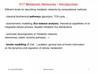
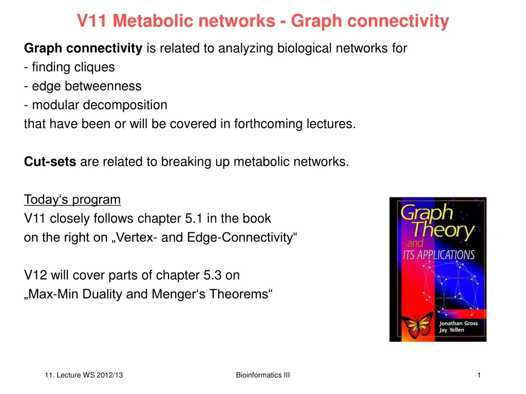
V11 Metabolic networks - Graph connectivity Graph connectivity is related to analyzing biological networks for - finding cliques - edge betweenness - modular decomposition that have been or will be covered in forthcoming lectures. Cut-sets are related to breaking up metabolic networks. Today‘s program V11 closely follows chapter 5.1 in the book on the right on „Vertex- and Edge-Connectivity“ V12 will cover parts of chapter 5.3 on „Max-Min Duality and Menger‘s Theorems“ Bioinformatics III
Citrate Cycle (TCA cycle) in E.coli Analysis of metabolic networks is at a relatively advanced/complete stage compared to protein-interaction networks or gene-regulatory networks. Possible reason: Most cellular metabolites are known. Bioinformatics III
Motivation – simple networks – task 1 What are all the possible steady-state flux distributions (v1, v2, v3, v4, v5, v6) in these networks? Bioinformatics III
Flux distributions: linear combinations of extreme pathways Compute extreme pathways („eigen vector basis“ of metabolic network): All 3 extreme pathways do not affect concentrations of internal metabolites. These are all extreme pathways of this network. All flux distributions in this network that can be written as linear combinations of these 3 extreme pathways are feasible steady-state flux distributions, but not others. Bioinformatics III
Motivation – simple networks – task 2 v1 – v7are the reaction fluxes of 7 reactions in this network that are catalyzed by transporters or enzymes 1 – 7. P is the product of interest of this network. What is the minimal number of reactions that need to be deleted (by gene knockouts or small molecule inhibitors) to block synthesis of P? Bioinformatics III
Characterize all minimal cut sets The system contains 6 elementary flux modes. 5 of them are coupled to synthesis of P. Each of these must be disconnected by deleting the smallest possible number of reactions find all minimal cut sets, take the smallest one. Bioinformatics III
Motivation: graph connectedness Some connected graphs are „more connected“ than others. E.g. some connected graphs can be disconnected by the removal of a single vertex or a single edge, whereas others remain connected unless more vertices or more edges are removed. use vertex-connectivity and edge-connectivity to measure the connectedness of a graph. Bioinformatics III
Motivation: graph connectedness Determining the number of edges (or vertices) that must be removed to disconnect a given connected graph applies directly to analyzing the vulnerability of existing networks. Definition: A graph is connected if for every pair of vertices u and v, there is a walk from u to v. Definition: A component of G is a maximal connected subgraph of G. Bioinformatics III
Vertex- and Edge-Connectivity Definition: A vertex-cut in a graph G is a vertex-set U such that G – U has more components than G. A cut-vertex (or cutpoint) is a vertex-cut consisting of a single vertex. Definition: An edge-cut in a graph G is a set of edges D such that G – D has more components than G. A cut-edge (or bridge) is an edge-cut consisting of a single edge. The vertex-connectivityv(G) of a connected graph G is the minimum number of vertices whose removal can either disconnect G or reduce it to a 1-vertex graph. if G has at least one pair of non-adjacent vertices, then v(G) is the size of a smallest vertex-cut. Bioinformatics III
Vertex- and Edge-Connectivity Definition: A graph G is k-connected if G is connected and v(G) ≥ k. If G has non-adjacent vertices, then G is k-connected if every vertex-cut has at least k vertices. Definition: The edge-connectivity e(G) of a connected graph G is the minimum number of edges whose removal can disconnect G. if G is a connected graph, the edge-connectivity e(G) is the size of a smallest edge-cut. Definition: A graph G is k-edge-connected if G is connected and every edge-cut has at least k edges (i.e. e(G) ≥ k). Bioinformatics III
Vertex- and Edge-Connectivity Example: In the graph below, the vertex set {x,y} is one of three different 2-element vertex-cuts. There is no cut-vertex. v(G) = 2. The edge set {a,b,c} is the unique 3-element edge-cut of graph G, and there is no edge-cut with fewer than 3 edges. Therefore e(G) = 3. Application: The connectivity measures v and e are used in a quantified model of network survivability, which is the capacity of a network to retain connections among its nodes after some edges or nodes are removed. Bioinformatics III
Vertex- and Edge-Connectivity Since neither the vertex-connectivity nor the edge-connectivity of a graph is affected by the existence or absence of self-loops, we will assume in the following that all graphs are loopless. Proposition 5.1.1 Let G be a graph. Then the edge-connectivity e(G) is less than or equal to the minimum degree min (G). Proof: Let v be a vertex of graph G with degree k = min(G). Then, the deletion of the k edges that are incident on vertex separates v from the other vertices of G. □ Bioinformatics III
Vertex- and Edge-Connectivity Definition: A collection of distinct non-empty subsets {S1,S2, ..., Sl} of a set A is a partition of A if both of the following conditions are satisfied: (1) Si∩ Sj = , 1 ≤ i < j ≤ l (2) i=1...l Si = A Definition: Let G be a graph, and let X1 and X2 form a partition of VG. The set of all edges of G having one endpoint in X1 and the other endpoint in X2 is called a partition-cut of G and is denoted X1,X2. Bioinformatics III
Partition Cuts and Minimal Edge-Cuts Proposition 4.6.3: Let X1,X2 be a partition-cut of a connected graph G. If the subgraphs of G induced by the vertex sets X1 and X2 are connected, then X1,X2 is a minimal edge-cut. Proof: The partition-cut X1,X2 is an edge-cut of G, since X1 and X2 lie in different components of G - X1,X2. Is it minimal? Let S be a proper subset of X1,X2, and let edge e X1,X2 - S. By definition of X1,X2, one endpoint of e is in X1 and the other endpoint is in X2. Thus, if the subgraphs induced by the vertex sets X1 and X2 are connected, then G – S is connected. Therefore, S is not an edge-cut of G, which implies that X1,X2 is a minimal edge-cut. □ Bioinformatics III
Partition Cuts and Minimal Edge-Cuts Proposition 4.6.4. Let S be a minimal edge-cut of a connected graph G, and let X1 and X2 be the vertex-sets of the two components of G – S. Then S = X1,X2. Proof: Clearly, S X1,X2, i.e. every edge e S has one endpoint in X1 and one in X2. Otherwise, the two endpoints would either both belong to X1 or to X2. Then, S would not be minimal because S – e would also be an edge-cut of G. On the other hand, if e X1,X2 - S, then its endpoints would lie in the same component of G – S, contradicting the definition of X1 and X2. □ Remark: This assumes that the removal of a minimal edge-cut from a connected graph creates exactly two components. Bioinformatics III
Partition Cuts and Minimal Edge-Cuts Proposition 4.6.5. A partition-cut X1,X2 in a connected graph G is a minimal edge-cut of G or a union of edge-disjoint minimal edge-cuts. Proof: Since X1,X2 is an edge-cut of G, it must contain a minimal edge-cut, say S. If X1,X2 S, then let e X1,X2 - S, where the endpoints v1 and v2 of e lie in X1 and X2, respectively. Since S is a minimal edge-cut, the X1-endpoints of S are in one of the components of G – S, and the X2-endpoints are in the other component. Furthermore, v1 and v2 are in the same component of G – S (since e G – S). Suppose, wlog, that v1 and v2 are in the same component as the X1-endpoints of S. Bioinformatics III
Partition Cuts and Minimal Edge-Cuts Then every path in G from v1 to v2 must use at least one edge of X1,X2 - S. Thus, X1,X2 - S is an edge-cut of G and contains a minimal edge-cut R. Appyling the same argument, X1,X2 - (S R) either is empty or is an edge-cut of G. Eventually, the process ends with X1,X2 - (S1 S2 ...Sr) = , where the Si are edge-disjoint minimal edge-cuts of G.□ Bioinformatics III
Partition Cuts and Minimal Edge-Cuts Proposition 5.1.2. A graph G is k-edge-connected if and only if every partition-cut contains at least k edges. Proof: () Suppose, that graph G is k-edge connected. Then every partition-cut of G has at least k edges, since a partition-cut is an edge-cut. () Suppose that every partition-cut contains at least k edges. By proposition 4.6.4., every minimal edge-cut is a partition-cut. Thus, every edge-cut contains at least k edges. □ Bioinformatics III
Relationship between vertex- and edge-connectivity Proposition 5.1.3. Let e be any edge of a k-connected graph G, for k≥ 3. Then the edge-deletion subgraph G – e is (k – 1)-connected. Proof: Let W = {w1, w2, ..., wk-2} be any set of k – 2 vertices in G – e, and let x and y be any two different vertices in (G – e) – W. It suffices to show the existence of an x-y walk in (G – e) – W. First, suppose that at least one of the endpoints of edge e is contained in set W. Since the vertex-deletion subgraph G – W is 2-connected, there is an x-y path in G – W. This path cannot contain edge e. Hence, it is an x-y path in the subgraph (G – e) – W. Next suppose that neither endpoint of edge e is in set W. Then there are two cases to consider. Bioinformatics III
Relationship between vertex- and edge-connectivity Case 1: Vertices x and y are the endpoints of edge e. Graph G has at least k + 1 vertices (since G is k-connected). So there exists some vertex z G – {w1,w2, ..., wk-2,x,y}. Since graph G is k-connected, there exists an x-z path P1 in the vertex deletion subgraph G – {w1,w2, ..., wk-2,y} and a z-y path P2 in the subgraph G – {w1,w2, ..., wk-2,x} Neither of these paths contains edge e, and, therefore, their concatenation is an x-y walk in the subgraph (G – e) – {w1,w2, ..., wk-2} Bioinformatics III
Relationship between vertex- and edge-connectivity Case 2: At least one of the vertices x and y, say x, is not an endpoint of edge e. Let u be an endpoint of edge e that is different from vertex x. Since graph G is k-connected, the subgraph G – {w1,w2, ..., wk-2,u} is connected. Hence, there is an x-y path P in G – {w1,w2, ..., wk-2,u}. It follows that P is an x-y path in G – {w1,w2, ..., wk-2} that does not contain vertex u and, hence excludes edge e (even if P contains the other endpoint of e, which it could). Therfore, P is an x-y path in (G – e) – {w1,w2, ..., wk-2}. □ Bioinformatics III
Relationship between vertex- and edge-connectivity Corollary 5.1.4. Let G be a k-connnected graph, and let D be any set of m edges of G, for m≤ k - 1. Then the edge-deletion subgraph G – D is (k – m)-connected. Proof: this follows from the iterative application of proposition 5.1.3. □ Corollary 5.1.5. Let G be a connected graph. Then e(G) ≥ v(G). Proof. Let k = v(G), and let S be any set of k – 1 edges in graph G. Since G is k-connected, the graph G – S is 1-connected, by corollary 5.1.4. Thus, the edge subset S is not an edge-cut of graph G, which implies that e(G) ≥ k. □ Corollary 5.1.6. Let G be a connected graph. Then v(G) ≤ e(G) ≤ min(G). This is a combination of Proposition 5.1.1 and Corollary 5.1.5. □ Bioinformatics III
Internally Disjoint Paths and Vertex-Connectivity:Whitney’s Theorem A communications network is said to be fault-tolerant if it has at least two alternative paths between each pair of vertices. This notion characterizes 2-connected graphs. A more general result for k-connected graphs follows later. Terminology: A vertex of a path P is an internal vertex of P if it is neither the initial nor the final vertex of that path. Definition: Let u and v be two vertices in a graph G. A collection of u-v paths in G is said to be internally disjoint if no two paths in the collection have an internal vertex in common. Bioinformatics III
Internally Disjoint Paths and Vertex-Connectivity:Whitney’s Theorem Theorem 5.1.7 [Whitney, 1932] Let G be a connected graph with n≥ 3 vertices. Then G is 2-connected if and only if for each pair of vertices in G, there are two internally disjoint paths between them. Proof: () Suppose that graph G is not 2-connected. Then let v be a cut-vertex of G. Since G – v is not connected, there must be two vertices such that there is no x-y path in G – v. It follows that v is an internal vertex of every x-y path in G. () Suppose that graph G is 2-connected, and let x and y be any two vertices in G. We use induction on the distance d(x,y) to prove that there are at least two vertex-disjoint x-y paths in G. If there is an edge e joining vertices x and y, (i.e., d(x,y) = 1), then the edge-deletion subgraph G – e is connected, by Corollary 5.1.4. Thus, there is an x-y path P in G – e. It follows that path P and edge e are two internally disjoint x-y paths in G. Bioinformatics III
Internally Disjoint Paths and Vertex-Connectivity:Whitney’s Theorem Next, assume for some k≥ 2 that the assertion holds for every pair of vertices whose distance apart is less than k. Let x and y be vertices such that distance d(x,y) = k, and consider an x-y path of length k. Let w be the vertex that immediately precedes vertex y on this path, and let e be the edge between vertices w and y. Since d(x,w) < k, the induction hypothesis implies that there are two internally disjoint x-w paths in G, say P and Q. Also, since G is 2-connected, there exists an x-y path R in G that avoids vertex w. Path Q either contains vertex y (right) or it does not (left) Bioinformatics III
Internally Disjoint Paths and Vertex-Connectivity:Whitney’s Theorem Let z be the last vertex on path R that precedes vertex y and is also on one of the paths P or Q (z might be vertex x). Assume wlog that z is on path P. Then G has two internally disjoint x-y paths. One of these paths is the concatenation of the subgraph of P from x to z with the subpath of R from z to y. If vertex y is not on path Q, then a second x-y path, internally disjoint from the first one, is the concatenation of path Q with the edge e joining vertex w to vertex y. If y is on path Q, then the subpath of Q from x to y can be used as the second path. □ Bioinformatics III
Internally Disjoint Paths and Vertex-Connectivity:Whitney’s Theorem Corollary 5.1.8. Let G be a graph with at least three vertices. Then G is 2-connected if and only if any two vertices of G lie on a common cycle. Proof: this follows from 5.1.7., since two vertices x and y lie on a common cycle if and only if there are two internally disjoint x-y paths.□ Bioinformatics III