Download
1 / 16
160 likes | 318 Vues
Hidden Process Models. Rebecca Hutchinson Tom M. Mitchell Indrayana Rustandi October 4, 2006 Women in Machine Learning Workshop Carnegie Mellon University Computer Science Department. Introduction. Hidden Process Models (HPMs): A new probabilistic model for time series data.

E N D
Hidden Process Models Rebecca Hutchinson Tom M. Mitchell Indrayana Rustandi October 4, 2006 Women in Machine Learning Workshop Carnegie Mellon University Computer Science Department
Introduction • Hidden Process Models (HPMs): • A new probabilistic model for time series data. • Designed for data generated by a collection of latent processes. • Potential domains: • Biological processes (e.g. synthesizing a protein) in gene expression time series. • Human processes (e.g. walking through a room) in distributed sensor network time series. • Cognitive processes (e.g. making a decision) in functional Magnetic Resonance Imaging time series.
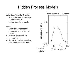
fMRI Data … Hemodynamic Response Features: 10,000 voxels, imaged every second. Training examples: 10-40 trials (task repetitions). Signal Amplitude Neural activity Time (seconds)
Study: Pictures and Sentences Press Button View Picture Read Sentence • Task: Decide whether sentence describes picture correctly, indicate with button press. • 13 normal subjects, 40 trials per subject. • Sentences and pictures describe 3 symbols: *, +, and $, using ‘above’, ‘below’, ‘not above’, ‘not below’. • Images are acquired every 0.5 seconds. Read Sentence Fixation View Picture Rest t=0 4 sec. 8 sec.
Goals for fMRI • To track cognitive processes over time. • Estimate process hemodynamic responses. • Estimate process timings. • Allowing processes that do not directly correspond to the stimuli timing is a key contribution of HPMs! • To compare hypotheses of cognitive behavior.
HPM Modeling Assumptions • Model latent time series at process-level. • Process instances share parameters based on their process types. • Use prior knowledge from experiment design. • Sum process responses linearly.
HPM Formalism HPM = <H,C,F,S> H = <h1,…,hH>, a set of processes (e.g. ReadSentence) h = <W,d,W,Q>, a process W = response signature d = process duration W = allowable offsets Q = multinomial parameters over values in W C = <c1,…, cC>, a set of configurations c = <p1,…,pL>, a set of process instances • = <h,l,O>, a process instance (e.g. ReadSentence(S1)) h = process ID • = timing landmark (e.g. stimulus presentation of S1) O = offset (takes values in Wh) • = <f1,…,fC>, priors over C S = <s1,…,sV>, standard deviation for each voxel
Process 1: ReadSentence Response signature W: Duration d: 11 sec. Offsets W: {0,1} P(): {q0,q1} Process 2: ViewPicture Response signature W: Duration d: 11 sec. Offsets W: {0,1} P(): {q0,q1} Processes of the HPM: v1 v2 v1 v2 Input stimulus : sentence picture Timing landmarks : Process instance:2 Process h: 2 Timing landmark: 2 Offset O: 1 (Start time: 2+ O) 1 2 One configuration c of process instances 1, 2, … k: (with prior fc) 1 2 Predicted mean: + N(0,s1) v1 v2 + N(0,s2)
HPMs: the graphical model Constraints from experiment design Timing Landmark l Process Type h Offset o Start Time s S p1,…,pk observed unobserved Yt,v t=[1,T], v=[1,V]
Algorithms • Inference • over configurations of process instances • choose most likely configuration with: • Learning • Parameters to learn: • Response signature W for each process • Timing distribution Q for each process • Standard deviation s for each voxel • Expectation-Maximization (EM) algorithm to estimate W and Q. • After convergence, use standard MLEs for s.
ViewPicture in Visual Cortex Offset q = P(Offset) 0 0.725 1 0.275
ReadSentence in Visual Cortex Offset q = P(Offset) 0 0.625 1 0.375
Decide in Visual Cortex Offset q = P(Offset) 0 0.075 1 0.025 2 0.025 3 0.025 4 0.225 5 0.625
Comparing Cognitive Hypotheses • Use cross-validation to choose a model. • GNB = HPM w/ ViewPicture, ReadSentence w/ d=8s. • HPM-2 = HPM w/ ViewPicture, ReadSentence w/ d=13s. • HPM-3 = HPM-2 + Decide Accuracy predicting picture vs. sentence (random = 0.5) Data log likelihood
Are we learning the right number of processes? • Use synthetic data where we know ground truth. • Generate training and test sets with 2/3/4 processes. • Train HPMs with 2/3/4 processes on each. • For each test set, select the HPM with the highest data log likelihood.
Conclusions • Take-away messages: • HPMs are a probabilistic model for time series data generated by a collection of latent processes. • In the fMRI domain, HPMs can simultaneously estimate the hemodynamic response and localize the timing of cognitive processes.