
Hidden Markov Models
Hidden Markov Models (HMMs) are statistical models that describe systems with hidden states. The Markov assumption posits that the current state is independent of past states, given the previous state. HMMs involve two key components: transition and observation models. Key inference tasks include filtering, smoothing, evaluation, and decoding. Filtering computes the probability of the current state given past evidence, while smoothing assesses past states based on full observation sequences. This guide explores HMM definitions, models, and practical applications.

Hidden Markov Models
E N D
Presentation Transcript
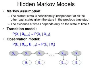
Hidden Markov Models • Markov assumption: • The current state is conditionally independent of all the other past states given the state in the previous time step • The evidence at time t depends only on the state at time t • Transition model: P(Xt | X0:t-1) = P(Xt | Xt-1) • Observation model: P(Et | X0:t, E1:t-1) = P(Et | Xt) … X2 Xt-1 Xt X0 X1 E2 Et-1 Et E1
An example HMM • States:X = {home, office, cafe} • Observations:E = {sms, facebook, email} Slide credit: Andy White
The Joint Distribution • Transition model: P(Xt | Xt-1) • Observation model: P(Et | Xt) • How do we compute the full joint P(X0:t, E1:t)? … X2 Xt-1 Xt X0 X1 E2 Et-1 Et E1
HMM inference tasks • Filtering: what is the distribution over the current state Xt given all the evidence so far, e1:t ? Query variable … … Xk Xt-1 Xt X0 X1 Ek Et-1 Et E1 Evidence variables
HMM inference tasks • Filtering: what is the distribution over the current state Xt given all the evidence so far, e1:t ? • Smoothing: what is the distribution of some state Xk given the entire observation sequence e1:t? … … Xk Xt-1 Xt X0 X1 Ek Et-1 Et E1
HMM inference tasks • Filtering: what is the distribution over the current state Xt given all the evidence so far, e1:t ? • Smoothing: what is the distribution of some state Xk given the entire observation sequence e1:t? • Evaluation: compute the probability of a given observation sequence e1:t … … Xk Xt-1 Xt X0 X1 Ek Et-1 Et E1
HMM inference tasks • Filtering: what is the distribution over the current state Xt given all the evidence so far, e1:t • Smoothing: what is the distribution of some state Xk given the entire observation sequence e1:t? • Evaluation: compute the probability of a given observation sequence e1:t • Decoding: what is the most likely state sequence X0:t given the observation sequence e1:t? … … Xk Xt-1 Xt X0 X1 Ek Et-1 Et E1
Filtering • Task: compute the probability distribution over the current state given all the evidence so far: P(Xt | e1:t) • Recursive formulation: suppose we know P(Xt-1 | e1:t-1) Query variable … … Xk Xt-1 Xt X0 X1 Ek Et-1 Et E1 Evidence variables
Filtering • Task: compute the probability distribution over the current state given all the evidence so far: P(Xt | e1:t) • Recursive formulation: suppose we know P(Xt-1 | e1:t-1) Time: t – 1 Time: t What is P(Xt = Office | e1:t-1) ? et-1 = Facebook 0.6 * 0.6 + 0.2 * 0.3 + 0.8 * 0.1=0.5 Home 0.6 Home ?? 0.6 0.2 Office 0.3 Office ?? 0.8 Cafe 0.1 Cafe ?? P(Xt | Xt-1) P(Xt-1 | e1:t-1)
Filtering • Task: compute the probability distribution over the current state given all the evidence so far: P(Xt | e1:t) • Recursive formulation: suppose we know P(Xt-1 | e1:t-1) Time: t – 1 Time: t What is P(Xt = Office | e1:t-1) ? et-1 = Facebook 0.6 * 0.6 + 0.2 * 0.3 + 0.8 * 0.1=0.5 Home 0.6 Home ?? 0.6 0.2 Office 0.3 Office ?? 0.8 Cafe 0.1 Cafe ?? P(Xt | Xt-1) P(Xt-1 | e1:t-1)
Filtering • Task: compute the probability distribution over the current state given all the evidence so far: P(Xt | e1:t) • Recursive formulation: suppose we know P(Xt-1 | e1:t-1) Time: t – 1 Time: t What is P(Xt = Office | e1:t-1) ? et-1 = Facebook 0.6 * 0.6 + 0.2 * 0.3 + 0.8 * 0.1=0.5 Home 0.6 Home ?? 0.6 0.2 Office 0.3 Office ?? 0.8 Cafe 0.1 Cafe ?? P(Xt | Xt-1) P(Xt-1 | e1:t-1)
Filtering • Task: compute the probability distribution over the current state given all the evidence so far: P(Xt | e1:t) • Recursive formulation: suppose we know P(Xt-1 | e1:t-1) Time: t – 1 Time: t What is P(Xt = Office | e1:t-1) ? et-1 = Facebook et = Email 0.6 * 0.6 + 0.2 * 0.3 + 0.8 * 0.1=0.5 Home 0.6 Home ?? 0.6 0.2 Office 0.3 Office ?? What is P(Xt = Office | e1:t) ? 0.8 Cafe 0.1 Cafe ?? P(Xt | Xt-1) P(et | Xt)= 0.8 P(Xt-1 | e1:t-1)
Filtering • Task: compute the probability distribution over the current state given all the evidence so far: P(Xt | e1:t) • Recursive formulation: suppose we know P(Xt-1 | e1:t-1) Time: t – 1 Time: t What is P(Xt = Office | e1:t-1) ? et-1 = Facebook et = Email 0.6 * 0.6 + 0.2 * 0.3 + 0.8 * 0.1=0.5 Home 0.6 Home ?? 0.6 0.2 Office 0.3 Office ?? What is P(Xt = Office | e1:t) ? 0.8 Cafe 0.1 Cafe ?? P(Xt | Xt-1) P(et | Xt)= 0.8 P(Xt-1 | e1:t-1)
Filtering • Task: compute the probability distribution over the current state given all the evidence so far: P(Xt | e1:t) • Recursive formulation: suppose we know P(Xt-1 | e1:t-1) Time: t – 1 Time: t What is P(Xt = Office | e1:t-1) ? et-1 = Facebook et = Email 0.6 * 0.6 + 0.2 * 0.3 + 0.8 * 0.1=0.5 Home 0.6 Home ?? 0.6 0.2 Office 0.3 Office ?? What is P(Xt = Office | e1:t) ? 0.8 Cafe 0.1 Cafe ?? 0.5*0.8= 0.4 Note: must also compute this value for Home and Cafe, and renormalize to sum to 1 P(Xt | Xt-1) P(et | Xt)= 0.8 P(Xt-1 | e1:t-1)
Filtering: The Forward Algorithm • Task: compute the probability distribution over the current state given all the evidence so far: P(Xt | e1:t) • Recursive formulation: suppose we know P(Xt-1 | e1:t-1) • Base case: priors P(X0) • Prediction: propagate belief from Xt-1 to Xt • Correction: weight by evidence et • Renormalize to have all P(Xt = x | e1:t) sum to 1
Filtering: The Forward Algorithm Time: 0 Time: t Time: t – 1 et-1 et Home prior … Home Home Office prior … Office Office Cafe prior … Cafe Cafe
Evaluation • Compute the probability of the current sequence: P(e1:t) • Recursive formulation: suppose we know P(e1:t-1)
Evaluation • Compute the probability of the current sequence: P(e1:t) • Recursive formulation: suppose we know P(e1:t-1) recursion filtering
Smoothing • What is the distribution of some state Xk given the entire observation sequence e1:t? … … Xk Xt-1 Xt X0 X1 Ek Et-1 Et E1
Smoothing • What is the distribution of some state Xk given the entire observation sequence e1:t? • Solution: the forward-backward algorithm Time: t Time: 0 Time: k et ek Home Home … Home … Office Office … Office … Cafe Cafe … Cafe … Forward message: P(Xk | e1:k) Backward message: P(ek+1:t | Xk)
Decoding: Viterbi Algorithm • Task: given observation sequence e1:t, compute most likely state sequence x0:t … … Xk Xt-1 Xt X0 X1 Ek Et-1 Et E1
Decoding: Viterbi Algorithm • Task: given observation sequence e1:t, compute most likely state sequence x0:t • The most likely path that ends in a particular state xt consists of the most likely path to some state xt-1 followed by the transition to xt Time: 0 Time: t Time: t – 1 xt-1 xt
Decoding: Viterbi Algorithm • Let mt(xt) denote the probability of the most likely path that ends in xt: Time: 0 Time: t Time: t – 1 P(xt| xt-1) xt-1 mt-1(xt-1) xt
Learning • Given: a training sample of observation sequences • Goal: compute model parameters • Transition probabilities P(Xt | Xt-1) • Observation probabilities P(Et | Xt) • What if we had complete data, i.e., e1:t and x0:t ? • Then we could estimate all the parameters by relative frequencies # of times state b follows state a P(Xt = b | Xt-1= a) total # of transitions from state a # of times e is emitted from state a P(E = e | X= a) total # of emissions from state a
Learning • Given: a training sample of observation sequences • Goal: compute model parameters • Transition probabilities P(Xt | Xt-1) • Observation probabilities P(Et | Xt) • What if we had complete data, i.e., e1:t and x0:t ? • Then we could estimate all the parameters by relative frequencies • What if we knew the model parameters? • Then we could use inference to find the posterior distribution of the hidden states given the observations
Learning • Given: a training sample of observation sequences • Goal: compute model parameters • Transition probabilities P(Xt | Xt-1) • Observation probabilities P(Et | Xt) • The EM (expectation-maximization) algorithm: • Starting with a random initialization of parameters: • E-step: find the posterior distribution of the hidden variables given observations and current parameter estimate • M-step: re-estimate parameter values given the expected values of the hidden variables


