Gravity Summary
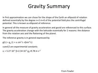
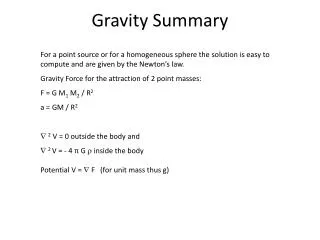
Gravity Summary. For a point source or for a homogeneous sphere the solution is easy to compute and are given by the Newton’s law. Gravity Force for the attraction of 2 point masses: F = G M 1 M 2 / R 2 a = GM / R 2 2 V = 0 outside the body and 2 V = - 4 π G inside the body

Gravity Summary
E N D
Presentation Transcript
Gravity Summary For a point source or for a homogeneous sphere the solution is easy to compute and are given by the Newton’s law. • Gravity Force for the attraction of 2 point masses: • F = G M1 M2 / R2 • a = GM / R2 • 2 V = 0 outside the body and • 2 V = - 4 π G inside the body • Potential V = F (for unit mass thus g)
Gravity Summary • This kind of forces and potential are typical for conservative field and follow the same rules that you have seen for the Electric field. In particular: • 2 V = 0 outside the body and • 2 V = - 4 π G inside the body. Are called Laplace and Poisson equations and are well known equations. The solution of the first equation are called harmonics.
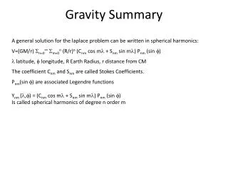
Gravity Summary A general solution for the laplace problem can be written in spherical harmonics: V=(GM/r) n=0∞ m=0n (R/r)n (Cnm cos m + Snm sin m) Pnm (sin ) latitude, longitude, R Earth Radius, r distance from CM The coefficient Cnm and Snm are called Stokes Coefficients. Pnm(sin ) are associated Legendre functions Ynm (,) = (Cnm cos m + Snm sin m) Pnm (sin ) Is called spherical harmonics of degree n order m
In general Cnm cos m Pnm (sin ) and Snm sin m Pnm (sin ) Are ortogonal functions => each function for a given degree and order can be thought of as contributing independent information with an amplitude given by their respective Cnm and Snm coefficients The zonal harmonics corresponding to m=0 have no longitude dependence and have n zeroes between +- 90 degrees in latitude So the even degree zonals are symmetric about the equator and the odd zonal are asymmetric. Note also that as the degree increases the number of zeroes in latitude increases and the harmonics represent finer latitudinal variations in the potential. If only large scale, such as the bulge, need to be modeled, then only the lowest degree zonal terms need to be used.
The nonzonal harmonics have longitudinal variations. The presence of the Cos m and sin m give the functions m zeroes in longitude And the Associated Legendre Functions have m zeroes in latitude. So similar to the zonals the higher degree and order harmonics represent finner spatial detail of the gravitational potential The nonzonal coefficients are called tesserals and for the specic case of n=m they are referred to as sectorials. Generally the spherical harmonics can be thought of as representing variations in the gravitational potential that have wavelengths of the circumference of the Earth divided by m in longitude and divided by n-m in latitude
http://en.wikipedia.org/wiki/Image:Harmoniques_spheriques_positif_negatif.pnghttp://en.wikipedia.org/wiki/Image:Harmoniques_spheriques_positif_negatif.png
Gravity Summary The coefficients are computed as: V=(GM/r) n=0∞ m=0n (R/r)n (Cnm cos m + Snm sin m) Pnm (sin ) the Stokes’ Coefficient up to n=2 have a clear physical meaning n=0: C=1 and S=0 so the first term of the spherical harmonics is only V= GM/r That is the gravity field of a point mass!
Gravity Summary V=(GM/r) n=0∞ m=0n (R/r)n (Cnm cos m + Snm sin m) Pnm (sin ) For n=1: C10 = zCM C11 = xCM S11 = yCM The Stokes coefficient are the coordinates of the Center of Mass. If the Center of Mass is the origin of our system they are zero!
Gravity Summary V=(GM/r) n=0∞ m=0n (R/r)n (Cnm cos m + Snm sin m) Pnm (sin ) For n=2: C20 = -1/(MR2) (I33- 0.5(I22+I11)) Difference diagonal term of inertia tensor C21 = I13/(MR2) S21 = I23/(MR2) C22 = (I22-I11)/(4MR2) S22 = I12/(2MR2) The max inertia axys is very close to the rotation axis z so I13 and I23 are small The other term are giving us the flattened shape of the Earth. Essentially the degree 2 of the spherical armonics are giving the correction to the potential due to the elliptical shape.
Often the potential is also written as a taylor expansion of the term r J is derived by precession of rotational axis or satellite orbits
Moment inertia homogeneous sphere: 2/5 MR2 ~ 0.4 MR2 For Earth ~0.3307 MR2 For Moon ~0.3935 MR2
Moment inertia homogeneous sphere: 2/5 MR2 ~ 0.4 MR2 For Earth ~0.3307 MR2 For Moon ~0.3935 MR2 The Earth has more mass close to the center The moon is almost homogeneous (max radius metallic core 300km) Mars: 0.366; Venus 0.33
Gravity Summary • In first approximation we can chose for the shape of the Earth an ellipsoid of rotation defined essentially by the degree n=2 m=0 of the potential field plus the centrifugal potential. This is known as ellipsoid of reference. • In general all the measure of gravity acceleration and geoid are referenced to this surface. The gravity acceleration change with the latitutde essentially for 2 reasons: the distance from the rotation axis and the flattening of the planet. • The reference gravity is in general expressed by • g() = ge (1 + sin2 +sin4 ) • and are experimental constants • = 5.27 10-3 =2.34 10-5 ge=9.78 m s-2 From Fowler
Gravity Summary A better approximation of the shape of the Earth is given by the GEOID. The GEOID is an equipotential surface corresponding to the average sea level surface From Fowler
H elevation over Geoid h elevation over ellipsoid N=h-H Local Geoid anomaly
Geoid Anomaly gΔh=-ΔV
Geoid Anomaly gΔh=-ΔV Dynamic Geoid