Download
1 / 27
270 likes | 414 Vues
Image Reconstruction from Non-Uniformly Sampled Spectral Data. Alfredo Nava-Tudela AMSC 664, Spring 2009 Final Presentation Advisor: John J. Benedetto. Signals and their spectral decomposition.

E N D
Image Reconstruction from Non-Uniformly Sampled Spectral Data Alfredo Nava-Tudela AMSC 664, Spring 2009 Final Presentation Advisor: John J. Benedetto AMSC 663/664
Signals and their spectral decomposition • A signal can be decomposed in harmonics that reveal the frequency or spectral content contained in that signal AMSC 663/664
Signals and their spectral decomposition • Often times, we have spectral information and we need to convert back to spatial information, for example Magnetic Resonance Imaging AMSC 663/664
Problem Statement • We are particularly interested in the reconstruction of images given spectral information • More specifically, we are interested in image reconstruction given non-uniformly sampled spectral data • Given a two dimensional spectral data set, reconstruct an image in the spatial domain that matches as closely as possible that data set in the spectral domain AMSC 663/664
The Algorithm • Stage one: AMSC 663/664
The Algorithm • Stage two: AMSC 663/664
The Algorithm • Stage three: Image Reconstructed AMSC 663/664
CG Experiments - Using the DFTxSinc input data AMSC 663/664
CG Experiments - Using the DFTxSinc input data AMSC 663/664
CG Experiments - Using the DFTxSinc input data AMSC 663/664
CG Experiments - Using the DFTxSinc input data AMSC 663/664
CG Experiments - Using the DFTxSinc input data AMSC 663/664
CG Experiments - Time of one iteration vs image size If N = 16 = 2^4, then ln(16)/ln(2) = 4. Time is given in seconds. AMSC 663/664
CG Experiments - Runtime vs Precision AMSC 663/664
CG Experiments - Number of iterations vs Precision AMSC 663/664
CG Experiments - Convergence and time results AMSC 663/664
CG Experiments - Convergence and time results The time is given in seconds AMSC 663/664
CG Experiments - Convergence and time results AMSC 663/664
CG Experiments - Convergence and time results The time is given in seconds AMSC 663/664
CG Experiments - Memory usage • One iteration of the CG method issues 2 calls to the function A_times() and 2 calls to the function A_star_times(). • Both functions, by implementation, use the same amount of memory. • The CG method also has bookkeeping variables that require memory. AMSC 663/664
CG Experiments - Memory usage A call to either A_times() or A_star_times() uses the following memory: Name Size Class Attributes KL N^2x2 double M 1x1 double N_square 1x1 double S Mx2 double a Mx1 double complex f N^2x1 double m 1x1 double n 1x1 double sum 1x1 double complex Which gives a sub-total for each call of: 3xN^2 + 4xM + 6 words AMSC 663/664
CG Experiments - Memory usage A call of the CG code, without the previous taken into account, uses the following memory: Name Size Class Attributes KL N^2x2 double S Mx2 double alpha 1x1 double complex beta 1x1 double d N^2x1 double complex delta_0 1x1 double delta_new 1x1 double delta_old 1x1 double f_hat Mx1 double complex iteration 1x1 double q N^2x1 double complex r N^2x1 double complex tol 1x1 double x N^2x1 double y N^2x1 double complex Which gives a sub-total of: 11xN^2 + 4xM + 8 words AMSC 663/664
CG Experiments - Memory usage Combined, we obtain the following grand total of: 14xN^2 + 8xM + 14 words needed to run our code. The direct method that saves the matrices A and its adjoint A* would need O(N^2 x M) words of memory. Clearly the CG method is the way to go memory wise! Direct Method CG Method We assume M = N^2, best case scenario AMSC 663/664
CG Experiments - Convergence N=16 AMSC 663/664
CG Experiments - Convergence N=32 AMSC 663/664
References • Richard F. Bass and Karlheinz Groechenig “Random Sampling of Multivariate Trigonometric Polynomials” • Zhou Wang, Alan C. Bovik, Hamid R. Sheikh, and Eero P. Simoncelli “Image Quality Assessment: From Error Measurements to Structural Similarity”, IEEE Transactions on Image Processing, Vol. 13, No. 1, January 2004 • Conjugate Gradient Method: http://en.wikipedia.org/wiki/Conjugate_gradient_method • Jonathan Richard Shewchuk, “An Introduction to the Conjugate Gradient Method Without the Agonizing Pain”. August 4, 1994. • Adi Ben-Israel and Thomas N. E. Greville. Generalized Inverses. Springer-Verlag, 2003. AMSC 663/664
References • John J. Benedetto and Paulo J. S. G. Ferreira. Moderm Sampling Theory: Mathematics and Applications. Birkhauser, 2001. • J. W. Cooley and J. W. Tukey. An algorithm for the machine computation of complex Fourier series. Math. Comp., 19:297-301, 1965. • E. H. Moore. On reciprocal of the general algebraic matrix. Bulletin of the American Mathematical Society, 26:85-100, 1920. • Diane P. O’Leary. Scientific computing with case studies. Book in preparation for publication, 2008. • Roger Penrose. On best approximate solution to linear matrix equations. Proceedings of the Cambridge Philosophical Society, 52:17-19, 1956. AMSC 663/664