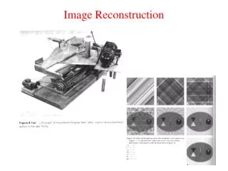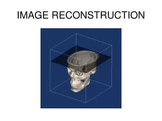
Statistical image reconstruction

1. Statistical image reconstruction MLEM (back) projection model OSEM MAP uniform resolution anatomical prior lesion detection

2. MLEM maximum likelihood expectation maximisation

3. Maximum Likelihood one wishes to find recon that maximizes p(recon | data) recon data computing p(recon | data) difficult inverse problem computing p(data | recon) “easy” forward problem Bayes: p(data | recon) p(recon) p(recon | data) = ~ p(data)

4. Maximum Likelihood p(recon | data) ~ p(data | recon) data recon projection Poisson lj p(data | recon) j = 1..J i = 1..I ln(p(data | recon)) = L(data | recon) = ~

5. Maximum Likelihood L(data | recon) find recon: Iterative inversion needed

6. Expectation Maximisation ML-EM algorithm: • produces non-negative solution • can be written as additive gradient ascent: • several useful alternative derivations exist

7. Expectation Maximisation likelihood l Optimisation transfer L(data | recon) L F In every iteration: = F(data | recon) lcurrent lnew lcurrent with L(data | lcurrent) = F(data | lcurrent)

8. Iterative Reconstruction likelihood iteration MEASUREMENT COMPARE UPDATE RECON REPROJECTION iteration

9. FBP vs MLEM h00189 FBP MLEM

10. FBP vs MLEM uniform Poisson

11. FBP vs MLEM Poisson Poisson FBP MLEM FBP MLEM uniform uniform

12. MLEM: non-uniform convergence 20 iterations 100 iterations True image Iteration sinogram

13. MLEM: non-uniform convergence 8 iter 100 iter FBP with noise smoothed true image sinogram

14. (back) projection model: model for image resolution

15. resolution model: simulation

16. resolution model: simulation no noise mlem Poisson noise mlem

17. resolution model: simulation no noise Poisson noise

18. resolution model: simulation no noise Poisson noise compute: estimated sinogram – given sinogram = “unexplained part of the data”

19. resolution model: simulation compute sum of squared differences along vertical lines

20. (back)projection in SPECT MLEM with single ray projector MLEM with Gaussian diffusion projector

21. (back)projection in PET 3D-PET FDG: OSEM, no resolution model 3D-PET FDG: OSEM, with resolution model

22. (back) projection model • accurate modeling of the physics: • larger fraction of the data becomes consistent •  better resolution • larger fraction of the noise becomes inconsistent •  less noise •  we gain twice! •  but computation time goes up...

23. OSEM ordered subsets expectation maximisation

24. OSEM 2 4 8 16 25 50 100 200 Reference Subsets... Filtered backprojection of the subsets.

25. OSEM 0 1 2 3 4 10 40 1 iteration of 40 subsets (2 proj per subset)

26. OSEM Reference 1 OSEM iteration with 40 subsets 0 1 2 3 4 10 40 0 1 2 3 4 10 40 MLEM-iterations

27. OSEM s1 s2 s3 s4 ML no noise (and subset balance) initial image with noise Convergence to limit cycle • Solutions: • apply converging block-iterative algorithm: • sacrifize some speed for guaranteed convergence • gradually decrease the number of subsets • ignore the problem (you may not want convergence anyway)

28. OSEM true 64x1 1x64 difference

29. MAP maximum a posteriori • short intro • MAP • uniform resolution • anatomical priors • lesion detection

30. MAP one wishes to find recon that maximizes p(recon | data) recon data computing p(recon | data) difficult inverse problem computing p(data | recon) “easy” forward problem Bayes: p(data | recon) p(recon) p(recon | data) = ~ p(data)

31. MAP j k Bayes: p(recon | data) ~ p(data | recon) p(recon) ln p(recon | data) ~ ln p(data | recon) + ln p(recon) prior posterior likelihood - penalty local prior or Markov prior: p(reconj | recon) = p(reconj | reconk, k is neighbor of j) Gibbs distribution: p(reconj | recon) = -bj Ej(Nj) + constant ln p(reconj | recon) =

32. MAP -bj Ej(Nj) ln p(reconj | recon) = E(lj – lk) quadratic Huber Geman lj – lk

33. MAP vssmoothed ML MLEM smoothed MLEM MAP with quadratic prior

34. MAP with uniform resolution • Likelihood provides non-uniform information: • some information is destroyed by • attenuation • Poisson noise • finite detector sensitivity and resolution • ... • Use non-uniform “prior” to smooth • more where likelihood is “strong” • less where likelihood is “weak” When postsmoothed-MLEM and MAP have same resolution, they have same covariance!

35. equivalent to post-smoothed MLEM prior improves condition number: MAP converges faster than MLEM: fewer iterations required! but more work per iteration MAP with uniform resolution

36. MAP with anatomical prior T1 Grey White CSF prior knowledge, valid for several tracer (FDG, ECD, ...) • CSF: no tracer uptake • white: uniform, low tracer uptake • grey: higher tracer uptake, • possibly lesions

37. MAP with anatomical prior MAP MRI MLEM • smoothing prior in gray matter (relative difference) • Intensity prior in white (with estimated mean) • Intensity prior in CSF (mean = 0)

38. MAP with anatomical prior Theoretical analysis indicates that PV-correction with MAP-reconstruction is superior to PV-correction with post-processed MLEM

39. MAP with anatomical prior map phantom sinogram map with anatomical prior and resolution modeling projection with finite resolution (2 pixels FWHM) make anatomical regions uniform ml-p ml with resolution modeling

40. MAP with anatomical prior map ml-p

41. MAP with anatomical prior MAP yields better noise characteristics than post-processed MLEM

42. MAP and lesion detection human observer study

43. MAP and lesion detection observer score human observer study MLEM MAP observer response time MLEM MAP human observer study more smoothing higher b more smoothing higher b

44. MAP and lesion detection observer score MLEM MAP MLEM MAP more smoothing higher b human observer study channelized Hotelling observer more smoothing higher b

45. MAP and lesion detection (non-uniform quadratic) MAP seems better for lesion detection

46. thanks