Statistical Methods for Image Reconstruction
Statistical Methods for Image Reconstruction. MIC 2007 Short Course October 30, 2007 Honolulu. Topics. Lecture I: Warming Up (Larry Zeng) Lecture II: ML and MAP Reconstruction (Johan Nuyts) Lecture III: X-Ray CT Iterative Reconstruction (Bruno De Man)


Statistical Methods for Image Reconstruction
E N D
Presentation Transcript
Statistical Methods for Image Reconstruction MIC 2007 Short Course October 30, 2007 Honolulu
Topics • Lecture I: Warming Up (Larry Zeng) • Lecture II: ML and MAP Reconstruction (Johan Nuyts) • Lecture III: X-Ray CT Iterative Reconstruction (Bruno De Man) • Round-Table Discussion of Your Interested Topics
Warming Up Larry Zeng, Ph.D. University of Utah
Continuous Unknown Image Problem to solve:Computed Tomography with discrete measurements Discrete Measurements
Continuous Unknown Image Analytic Algorithms • For example, FBP (Filtered Backprojection) • Treat the unknown image as continuous • Point-by-point reconstruction (arbitrary points) • Regular grid points are commonly chosen for display
Iterative Algorithms • For example, ML-EM, OS-EM, ART, GC, … • Discretize the image into pixels • Solve imaging equations AX=P • X = unknowns (pixel values) • P = projection data • A = imaging system matrix P aij X
p1 p2 x1 x2 p3 x3 x4 p4 Example AX=P
Example 5 4 x1 x2 3 • AX=P • Rank(A) = 3 < 4 • System not consistent • No solution x3 x4 2
Solving AX=P • In practice, A is not invertible (not square, or not full rank) • A generalized inverse is used X = A†P • Moore-Penrose inverse A†=(ATA)-1AT AA†A=A A†AA†=A† Least-squares solution (Gaussian noise model)
Least-squares solution 4 3 5 4 3 4 2.25 1.75 2 3 1.75 1.25
The most significant motivation of using an iterative algorithm:Usually, iterative algorithms give better reconstructions than analytical algorithms.
Computer Simulations Examples (Fessler) FBP = Filtered Backprojection (Analytical) PWLS = Penalized data-weighted least squares (Iterative) PL (or MAP) = Penalized likelihood (Iterative)
Why are iterative algorithms better than analytical algorithms? • The system matrix A is more flexible than the assumptions in an analytical algorithm • It is a lot harder for an analytical algorithm to handle some realistic situations
Attenuation in SPECT • Photon attenuation is spatially variant • Non-uniform atten. modeled in an iterative algorithm system matrix A (1970s) • Uniform atten. in analytic algorithm (1980s) • Non-uniform atten. in analytic algorithm (2000s)
Distance-Dependent Blurring Close Far
Distance-Dependent Blurring • System matrix A models the blurring P X
Near Far Distance-Dependent Blurring • Analytic treatment uses the Frequency-Distance Principle (approximation) Near Far Slope ~ Distance
Truncation • (Analytic) Old FBP algorithm does not allow truncation • (Iterative) System matrix only models measured data, ignores unmeasured data • (Analytic) New DBP (Derivative Backprojection) algorithm can handle some truncation situations
Scatter Scattered Primary
Scatter • (Iterative) System matrix A can model scatter using “effective scattering source” or Monte Carlo • (Analytic) Still don’t know how, other than preprocessing data using multiple energy windows
In physics and imaging geometry modeling, analytic methods are behind the iterative ones.
Data Filtering Image Backprojection Analytic algorithm — “Open-loop system”
Iterative algorithm — “Closed-loop system” Compare Image Projection Data A AT Update Backprojection
Main Difference • Analytic algorithms do not have a projector A, but have a set of assumptions. • Iterative algorithms have a projector A.
Under what conditions will the analytic algorithm outperform the iterative algorithm? • The analytical assumptions (e.g., sampling, geometry, physics) • System matrix A is always an approximation (e.g., the pixel model assumes a uniform activity within the pixel)
Noise Consideration • Iterative: Objective function (e.g., Likelihood) • Iterative: Regularization (very effective!) • Analytic: Filtering (assumes spatially invariant, not as good)
Modeling noise in an iterative algorithm (thus Statistical Algorithm) Example: A one-pixel image (i.e., total count is the only concern) 3 measurements: • 1100 counts for 10 sec. (110/s) • 100 counts for 1 sec. (100/s) • 15000 counts for 100 sec. (150/s) Counts per second?
m1 = 1100, s2(m1)=1100, x1=1100/10=110, s2(x1)= s2(m1)/(10)2 = 1100/100=11 m2 = 100, s2(m2)=100, x2=100/1=10, s2(x2)= s2(m2)= 100 m3 = 15000, s2(m3)=15000, x3=15000/100=150, s2(x3)= s2(m3)/(100)2 = 15000/10000=1.5
Generalization • If you have N unknowns, you need to make a lot more than N measurements. • The measurements are redundant. • Put more weights on the measurements that you trust more.
Geometric Illustration • Two unknowns x1, x2 • Each measurement = a linear eqn = 1 line • We make 3 measurements; we have 3 lines
Noise Free (consistent) x2 x1
Noisy (inconsistent) x2 e2 e3 e1 x1
If you don’t have redundant measurements, the noise model (e.g., s2) does not make any differences x2 x1
In practice, # of unknowns ≈ # of measurements • However, iterative methods still outperform analytic methods • Why?
Answer: Regularization & Constraints • Helpful constraints: Non-negativity (xi≥ 0) Image support (xk = 0, x inK) Bounds of values (e.g. transmission map) • Prior
Some common regularization methods (1) — Stop early • Why stop? Doesn’t the algorithm converge? • Yes, in many cases (e.g., ML-EM) it does. • When an ML-EM reconstruction becomes noisy, its likelihood function is still increasing. • The ultimate solution (e.g., ML-EM) solution is too noisy; we don’t like it.
Iterative Reconstruction An Example (ML-EM)
Iterative Reconstruction An Example (ML-EM)
Iterative Reconstruction An Example (ML-EM)
Iterative Reconstruction An Example (ML-EM)
Iterative Reconstruction An Example (ML-EM)
Iterative Reconstruction An Example (ML-EM)
Iterative Reconstruction An Example (ML-EM)
Iterative Reconstruction An Example (ML-EM)
EARLY • Stopping early is like lowpass filtering. • Low freq. components converge faster than high freq. components.
Regularization using Prior What is a prior? Example: • You want to estimate tomorrow’s temperature. • You know today’s temperature. • You assume that tomorrow’s temperature is pretty close to today’s