Image Restoration and Reconstruction (Linear Restoration Methods)
700 likes | 1.23k Vues
Digital Image Processing. Image Restoration and Reconstruction (Linear Restoration Methods). Christophoros Nikou cnikou@cs.uoi.gr. Contents. In this lecture we will look at linear image restoration techniques Differentiation of matrices and vectors Linear space invariant degradation

Image Restoration and Reconstruction (Linear Restoration Methods)
E N D
Presentation Transcript
Digital Image Processing Image Restoration and Reconstruction(Linear Restoration Methods) Christophoros Nikou cnikou@cs.uoi.gr
Contents In this lecture we will look at linear image restoration techniques • Differentiation of matrices and vectors • Linear space invariant degradation • Restoration in absence of noise • Inverse filter • Pseudo-inverse filter • Restoration in presence of noise • Inverse filter • Wiener filter • Constrained least squares filter
Differentiation of Matrices and Vectors Notation: A is a MxN matrix with elements aij. x is a Nx1 vector with elements xi. f(x)is a scalar function of vector x. g(x)is a Mx1 vector valued function of vector x.
Differentiation of Matrices and Vectors (cont...) Scalar derivative of a matrix. A is a MxN matrix with elements aij.
Differentiation of Matrices and Vectors (cont...) Vector derivative of a function (gradient). x is a Nx1 vector with elements xi. f(x)is a scalar function of vector x.
Differentiation of Matrices and Vectors (cont...) Vector derivative of a vector (Jacobian): x is a Nx1 vector with elements xi. g(x)is a Mx1 vector valued function of vector x.
Differentiation of Matrices and Vectors (cont...) Some useful derivatives. x is a Nx1 vector with elements xi. b is a Nx1 vector with elements bi. It is the derivative of the scalar valued function bTx with respect to vector x.
Differentiation of Matrices and Vectors (cont...) Some useful derivatives. x is a Nx1 vector with elements xi. A is a MxN matrix with elements aij. If A is symmetric:
Differentiation of Matrices and Vectors (cont...) Some useful derivatives. x is a Nx1 vector with elements xi. b is a Nx1 vector with elements bi. A is a MxN matrix with elements aij. It may be proved using the previous properties.
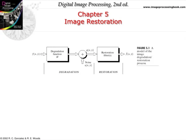
Linear, Position-Invariant Degradation We now consider a degraded image to be modelled by: where h(x, y) is the impulse response of the degradation function ( i.e. point spread function blurringthe image). The convolution implies that the degradation mechanism is linear and position invariant (it depends only on image values and not on location).
Linear, Position-Invariant Degradation (cont...) In the Fourier domain: where multiplication is element-wise. In matrix-vector form: where H is a doubly block circulant matrix and f,g, andηare vectors (lexicographic ordering).
Linear, Position-Invariant Degradation (cont...) If the degradation function is unknown the problem of simultaneously recovering f(x,y) and h(x,y) is called blind deconvolution.
Linear Restoration Using the imaging system we want to estimate the true image from the degraded observation with known degradation H. A linear method applies an operator (a matrix) P to the observation g to estimate the unobserved noise-free image f:
Restoration in Absence of NoiseThe Inverse Filter When there is no noise: an obvious solution would be to use the inverse filter: yielding
Restoration in Absence of NoiseThe Inverse Filter (cont...) For a NxN image, H is a N2xN2 matrix! To tackle the problem we transform it to the Fourier domain. H is doubly block circulant and therefore it may be diagonalized by the 2D DFT matrix W:
Restoration in Absence of NoiseThe Inverse Filter (cont...) where Therefore:
Restoration in Absence of NoiseThe Inverse Filter (cont...) Which is the vectorized form of the DFT of the image: Take the inverse DFT and obtain f(m,n). Problem: what happens if H(k,l) has zero values? Cannot perform inverse filtering!
Restoration in Absence of NoiseThe Pseudo-inverse Filter A solution is to set: which is a type of pseudo-inversion. Notice that the signal cannot be restored at locations where H(k,l)=0.
Restoration in Absence of NoiseThe Pseudo-inverse Filter (cont...) A pseudo-inverse filter also arises by the unconstrained least squares approach. Find the image f, that, when it is blurred by H, it will provide an observation as close as possible to g, i.e. It minimizes the distance between Hf and g.
Restoration in Absence of NoiseThe Pseudo-inverse Filter (cont...) This distance is expressed by the norm:
Restoration in Presence of NoiseThe Inverse Filter Recall the imaging model with spatially invariant degradation and noise
Restoration in Presence of NoiseThe Inverse Filter (cont...) Applying the inverse filter in the Fourier domain: Even if we know H(k,l) we cannot recover F(k,l) due to the second term. If H(k,l) has small values the second term dominates (it goes to infinity if H(k,l)=0!).
Restoration in Presence of NoiseThe Inverse Filter (cont...) One approach to get around the problem is to limit the ratio G(k,l) / H(k,l) to frequencies near the origin that have lower probability of being zero. We know that H(0,0) is usually the highest value of the DFT. Thus, by limiting the analysis to frequencies near the origin we reduce the probability of encountering zero values.
Restoration in Presence of NoiseThe Inverse Filter (cont...) Blurring degradation
Restoration in Presence of NoiseThe Inverse Filter (cont...) Inverse filter with cut-off
Restoration in Presence of NoiseWiener Filter So far we assumed nothing about the statistical properties of the image and noise. We now consider image and noise as random variables and the objective is to find an estimate of the uncorrupted image f such that the mean square error between the estimate and the image is minimized: where E[x] is the expected value of vector x.
Restoration in Presence of NoiseWiener Filter (cont...) Recall also the definition of the correlation matrix between two vectors x and y: We assume that the image and the noise are uncorrelated:
Restoration in Presence of NoiseWiener Filter (cont...) We are looking for the best estimate: Let’s confine our estimate to be obtainable by a linear operator on the observation: and the goal is to find the best matrix P.
Restoration in Presence of NoiseWiener Filter (cont...) Denoting by the n-th row of P:
Restoration in Presence of NoiseWiener Filter (cont...) We can now minimize the sum with respect to each term:
Restoration in Presence of NoiseWiener Filter (cont...) Assembling the rows together: We have to compute the two matrices:
Restoration in Presence of NoiseWiener Filter (cont...) Assumming noise is uncorrelated with image: Also, Finally the matrix we are looking for is
Restoration in Presence of NoiseWiener Filter (cont...) The estimated uncorrupted image is which may be also expressed as This result is known as the Wiener filter or the minimum mean square error (MMSE) filter.
Restoration in Presence of NoiseWiener Filter (cont...) Special cases: No blur (H=I, g=f+η): No noise (Rηη=0, g=Ηf): This is the inverse filter. No blur, no noise (H=I, Rηη=0): Do nothing on the observation.
Restoration in Presence of NoiseWiener Filter (cont...) The size of the matrix to be inverted poses difficulties and Wiener filter is implemented in the Fourier domain. This occurs when H is doubly block circulant (represents convolution) and the image f and noise η are wide-sense stationary (w.s.s). Definition of a w.s.s. signal: 1) E[f(m,n)]=μ, independent of m,n. 2) E[f(m,n)f(k,l)]=r(m-k,n-l), independent of location.
Restoration in Presence of NoiseWiener Filter (cont...) Reminder: the inverse DFT complex exponential matrix diagonalizes any circulant matrix: The columns of W-1 are the eigenvectors of any circulant matrix H. The corresponding eigenvalues are the DFT values of the signal producing the circulant matrix. Remember also that and that
Restoration in Presence of NoiseWiener Filter (cont...) We will employ the following relations: If H is real:
Restoration in Presence of NoiseWiener Filter (cont...) The Wiener solution is now transformed to the Fourier domain: Notice that the matrices are diagonal.
Restoration in Presence of NoiseWiener Filter (cont...) Sff (k,l)=DFT(Rff (m,n)) is the power spectrum of the image f (m,n). Sηη(k,l)=DFT(Rηη(m,n)) is the power spectrum of the noiseη(m,n).
Restoration in Presence of NoiseWiener Filter (cont...) If Sff (k,l) is not zero we may define the Signal to Noise Ratio in the frequency domain: and the Wiener filter becomes:
Restoration in Presence of NoiseWiener Filter (cont...) A well known estimate of Sff (k,l) is the periodogram (the ML estimate of Rffwhen f ia assumed Gaussian): In practice, as F(k,l) is unknown, we use
Restoration in Presence of NoiseWiener Filter (cont...) Wiener Inverse Degraded image Noise variance one order of magnitude less. Noise variance ten orders of magnitude less.
Restoration in Presence of NoiseConstrained Least Squares Filter When we do not have information on the power spectra the Wiener filter is not optimal. Another idea is to introduce a smoothness term in our criterion. We define smoothness by the quantity where Q is a high pass filter operator, e.g. the Laplacian, (Q is a doubly block circulant matrix representing convolution by the Laplacian). We look for smooth solutions minimizing
Restoration in Presence of NoiseConstrained Least Squares Filter (cont...) We have the following constrained least squares (CLS) optimization problem: Minimize subject to yielding the Lagrange multiplier minimization of the function: Smoothness term Data fidelity term
Restoration in Presence of NoiseConstrained Least Squares Filter (cont...) Parameter λ controls the degree of smothness: pseudo-inverse, ultra rough solution ultra smooth solution
Restoration in Presence of NoiseConstrained Least Squares Filter (cont...) In the Fourier domain, the constrained least squares filter becomes: Keep always in mind to zero-pad the images properly.
Restoration in Presence of NoiseConstrained Least Squares Filter (cont...) Low noise: Wiener and CLS generate equal results. High noise: CLS outperforms Wiener if λ is properly selected. It is easier to select the scalar value for λ than to approximate the SNR which is seldom constant.
Restoration Performance Measures Original image f and restored image Mean square error (MSE):
