Image Restoration and Denoising
390 likes | 979 Vues
Image Restoration and Denoising. Chapter Seven – Part II. Image Restoration Techniques. Inverse of degradation process Depending on the knowledge of degradation, it can be classified into. Image Restoration Model. f’(x,y). η (x, y). Image Restoration Model. In this model,

Image Restoration and Denoising
E N D
Presentation Transcript
Image Restoration and Denoising Chapter Seven – Part II
Image Restoration Techniques • Inverse of degradation process • Depending on the knowledge of degradation, it can be classified into
Image Restoration Model f’(x,y) η (x, y)
Image Restoration Model • In this model, • f(x,y) input image • h(x,y) degradation • f'(x,y) restored image • η(x,y) additive noise • g(x,y) degraded image
Image Restoration Model • In spatial domain, g(x,y) = f(x,y) * h(x,y) and in frequency domain G(k,l) = F(k,l). H(k,l) Where G,F and H are fourier transform of g,f and h
Linear Restoration Technique • They are quick and simple • But limited capabilities • It includes • Inverse Filter • Pseudo Inverse Filter • Wiener Filter • Constrained Least Square Filter
Inverse Filtering • If we know exact PSF and ignore noise effect, this approach can be used. • In practice PSF is unknown and degradation is affected by noise and hence this approach is not perfect. • Advantage - Simple
Inverse Filtering • From image restoration model • For simplicity, the co-ordinate of the image are ignored so that the above equation becomes • Then the error function becomes
Inverse Filtering • We wish to ignore η and use to approximate under least square sense. Then the error function is given as • To find the minimum of , the above equation is differentiated wrt and equating it to zero
Inverse Filtering • Solving for , we get • Taking fourier transform on both sides we get • The restored image in spatial domain is obtained by taking Inverse Fourier Transform as
Inverse Filtering • Advantages: • It requires only blur PSF • It gives perfect reconstruction in the absence of noise • Drawbacks: • It is not always possible to obtain an inverse (singular matrices) • If noise is present, inverse filter amplifies noise. (better option is wiener filter)
Pseudo-Inverse Filtering • For an inverse filter, • Here H(k,l) represents the spectrum of the PSF. • The division of H(k,l) leads to large amplification at high frequencies and thus noise dominates over image
Pseudo-Inverse Filtering • To avoid this problem, a pseudo-inverse filter is defined as • The value of ε affects the restored image • With no clear objective selection of ε, the restored images are generally noisy and not suitable for further analysis
SVD Approach for Pseudo-Inverse Filtering • SVD stands for Singular Value Decomposition • Using SVD any matrix can be decomposed into a series of eigen matrices • From image restoration model we have • The blur matrix is represented by H • H is decomposed into eigen matrices as where U and V are unitary and D is diagonal matrix
SVD Approach for Pseudo-Inverse Filtering • Then the pseudo inverse of H is given by • The generalized inverse is the estimate is the result of multiplying H† with g • R indicates the rank of the matrix • The resulting sequence estimation formula is given as
SVD Approach for Pseudo-Inverse Filtering • Advantage • Effective with noise amplification problem as we can interactively terminate the restoration • Computationally efficient if noise is space invariant • Disadvantage • Presence of noise can lead to numerical instability
Wiener Filter • The objective is to minimize the mean sqaure error • It has the capability of handling both the degradation function and noise • From the restoration model, the error between input image f(m,n) and the estimated image is given by
Wiener Filter • The square error is given by • The mean square error is given by
Wiener Filter • The objective of the Wiener filter is top minimize • Given a system we have y=h*x + v h-blur function x - original image y – observed image (degraded image) v – additive noise
Wiener Filter • The goal is to obtain g such that is the restored image that minimizes mean square error • The deconvolution provides such a g(t)
Wiener Filter • The filter is described in frequency domain as • G and H are fourier transform of g and h • S – mean power of spectral density of x • N – mean power of spectral density of v • * - complex conjugate
Wiener Filter • Drawback – It requires prior knowledge of power spectral density of image which is unavailable in practice