Where to leave the data ? Parallel systems Scalable Distributed Data Structures
Where to leave the data ? Parallel systems Scalable Distributed Data Structures Dynamic Hash Table (P2P). Parallel machines are quite common and affordable Databases are growing increasingly large large volumes of transaction data are collected and stored for later analysis.

Where to leave the data ? Parallel systems Scalable Distributed Data Structures
E N D
Presentation Transcript
Where to leave the data ? • Parallel systems • Scalable Distributed Data Structures • Dynamic Hash Table (P2P)
Parallel machines are quite common and affordable Databases are growing increasingly large large volumes of transaction data are collected and stored for later analysis. multimedia objects like images are increasingly stored in databases Large-scale parallel database systems increasingly used for: storing large volumes of data processing time-consuming decision-support queries providing high throughput for transaction processing Introduction
Data can be partitioned across multiple disks for parallel I/O. Individual relational operations (e.g., sort, join, aggregation) can be executed in parallel data can be partitioned and each processor can work independently on its own partition. Queries are expressed in high level language (SQL, translated to relational algebra) makes parallelization easier. Different queries can be run in parallel with each other. Concurrency control takes care of conflicts. Thus, databases naturally lend themselves to parallelism. Parallelism in Databases
Reduce the time required to retrieve relations from disk by partitioning the relations on multiple disks. Horizontal partitioning – tuples of a relation are divided among many disks such that each tuple resides on one disk. Partitioning techniques (number of disks = n): Round-robin: Send the ith tuple inserted in the relation to disk i mod n. Hash partitioning: Choose one or more attributes as the partitioning attributes. Choose hash function h with range 0…n - 1 Let i denote result of hash function h applied to the partitioning attribute value of a tuple. Send tuple to disk i. I/O Parallelism
Partitioning techniques (cont.): Range partitioning: Choose an attribute as the partitioning attribute. A partitioning vector [vo, v1, ..., vn-2] is chosen. Let v be the partitioning attribute value of a tuple. Tuples such that vivi+1 go to disk I + 1. Tuples with v < v0 go to disk 0 and tuples with v vn-2 go to disk n-1. E.g., with a partitioning vector [5,11], a tuple with partitioning attribute value of 2 will go to disk 0, a tuple with value 8 will go to disk 1, while a tuple with value 20 will go to disk2. I/O Parallelism (Cont.)
Evaluate how well partitioning techniques support the following types of data access: 1.Scanning the entire relation. 2.Locating a tuple associatively – point queries. E.g., r.A = 25. 3.Locating all tuples such that the value of a given attribute lies within a specified range – range queries. E.g., 10 r.A < 25. Comparison of Partitioning Techniques
Round robin: Advantages Best suited for sequential scan of entire relation on each query. All disks have almost an equal number of tuples; retrieval work is thus well balanced between disks. Range queries are difficult to process No clustering -- tuples are scattered across all disks Comparison of Partitioning Techniques (Cont.)
Hash partitioning: Good for sequential access Assuming hash function is good, and partitioning attributes form a key, tuples will be equally distributed between disks Retrieval work is then well balanced between disks. Good for point queries on partitioning attribute Can lookup single disk, leaving others available for answering other queries. Index on partitioning attribute can be local to disk, making lookup and update more efficient No clustering, so difficult to answer range queries Comparison of Partitioning Techniques(Cont.)
Range partitioning: Provides data clustering by partitioning attribute value. Good for sequential access Good for point queries on partitioning attribute: only one disk needs to be accessed. For range queries on partitioning attribute, one to a few disks may need to be accessed Remaining disks are available for other queries. Good if result tuples are from one to a few blocks. If many blocks are to be fetched, they are still fetched from one to a few disks, and potential parallelism in disk access is wasted Example of execution skew. Comparison of Partitioning Techniques (Cont.)
If a relation contains only a few tuples which will fit into a single disk block, then assign the relation to a single disk. Large relations are preferably partitioned across all the available disks. If a relation consists of m disk blocks and there are n disks available in the system, then the relation should be allocated min(m,n) disks. Partitioning a Relation across Disks
The distribution of tuples to disks may be skewed— that is, some disks have many tuples, while others may have fewer tuples. Types of skew: Attribute-value skew. Some values appear in the partitioning attributes of many tuples; all the tuples with the same value for the partitioning attribute end up in the same partition. Can occur with range-partitioning and hash-partitioning. Partition skew. With range-partitioning, badly chosen partition vector may assign too many tuples to some partitions and too few to others. Less likely with hash-partitioning if a good hash-function is chosen. Handling of Skew
To create a balanced partitioning vector (assuming partitioning attribute forms a key of the relation): Sort the relation on the partitioning attribute. Construct the partition vector by scanning the relation in sorted order as follows. After every 1/nth of the relation has been read, the value of the partitioning attribute of the next tuple is added to the partition vector. n denotes the number of partitions to be constructed. Duplicate entries or imbalances can result if duplicates are present in partitioning attributes. Alternative technique based on histograms used in practice Handling Skew in Range-Partitioning
Handling Skew using Histograms • Balanced partitioning vector can be constructed from histogram in a relatively straightforward fashion • Assume uniform distribution within each range of the histogram • Histogram can be constructed by scanning relation, or sampling (blocks containing) tuples of the relation
Handling Skew Using Virtual Processor Partitioning • Skew in range partitioning can be handled elegantly using virtual processor partitioning: • create a large number of partitions (say 10 to 20 times the number of processors) • Assign virtual processors to partitions either in round-robin fashion or based on estimated cost of processing each virtual partition • Basic idea: • If any normal partition would have been skewed, it is very likely the skew is spread over a number of virtual partitions • Skewed virtual partitions get spread across a number of processors, so work gets distributed evenly! /ufs/mk/monet5/Linux/mTests/
Scalable Distributed Data Structures • The leading researcher is Withold Litwin
Why SDDSs • Multicomputers need data structures and file systems • Trivial extensions of traditional structures are not best • hot-spots • scalability • parallel queries • distributed and autonomous clients • distributed RAM & distance to data
What is an SDDS ? • Data are structured • records with keys objects with an OID • more semantics than in Unix flat-file model • abstraction popular with applications • allows for parallel scans • function shipping • Data are on servers • always available for access • Overflowing servers split into new servers • appended to the file without informing the clients • Queries come from multiple autonomous clients • available for access only on their initiative • no synchronous updates on the clients • There is no centralized directory for access computations
What is an SDDS ? • Clients can make addressing errors • Clients have less or more adequate image of the actual file structure • Servers are able to forward the queries to the correct address • perhaps in several messages • Servers may send Image Adjustment Messages • Clients do not make same error twice • See the SDDS talk for more on it • http://ceria.dauphine.fr/witold.html • Or the LH* ACM-TODS paper (Dec. 96)
An SDDS growth through splits under inserts Servers Clients
An SDDS growth through splits under inserts Servers Clients
An SDDS growth through splits under inserts Servers Clients
An SDDS growth through splits under inserts Servers Clients
An SDDS growth through splits under inserts Servers Clients
An SDDS Clients
An SDDS Clients
An SDDS IAM Clients
An SDDS Clients
An SDDS Clients
k-RP* dPi-tree Nardelli-tree RP* Kroll & Widmayer Breitbart & Vingralek Known SDDSs DS SDDS (1993) Classics m-d trees Hash 1-d tree LH* DDH Breitbart & al H-Avail. LH*m, LH*g LH*SA Security s-availability LH*s LH*RS
LH* (A classic) • Allows for the primary key (OID) based hash files • generalizes the LH addressing schema • variants used in Netscape products, LH-Server, Unify, Frontpage, IIS, MsExchange... • Typical load factor 70 - 90 % • In practice, at most 2 forwarding messages • regardless of the size of the file • In general, 1 m/insert and 2 m/search on the average • 4 messages in the worst case • Search time of 1 ms (10 Mb/s net), of 150 s (100 Mb/s net) and of 30 s (Gb/s net)
High-availability LH* schemes • In a large multicomputer, it is unlikely that all servers are up • Consider the probability that a bucket is up is 99 % • bucket is unavailable 3 days per year • If one stores every key in only 1 bucket • case of typical SDDSs, LH* included • Thenfile reliability : probability that n-bucket file is entirely up is: • 37 % for n = 100 • 0 % for n = 1000 • Acceptable for yourself ?
High-availability LH* schemes • Using 2 buckets to store a key, one may expect the reliability of: • 99 % for n = 100 • 91 % for n = 1000 • High-availability files • make data available despite unavailability of some servers • RAIDx, LSA, EvenOdd, DATUM... • High-availability SDDS • make sense • are the only way to reliable large SDDS files
Chord lookup algorithm properties • Interface: lookup(key) IP address • Efficient: O(log N) messages per lookup • N is the total number of servers • Scalable: O(log N) state per node • Robust: survives massive failures • Simple to analyze
Chord Hashes a Key to its Successor Key ID Node ID N10 K5, K10 K100 N100 Circular ID Space N32 K11, K30 K65, K70 N80 N60 K33, K40, K52 • Successor: node with next highest ID
Basic Lookup N5 N10 N110 “Where is key 50?” N20 N99 “Key 50 is At N60” N32 N40 N80 N60 • Lookups find the ID’s predecessor • Correct if successors are correct
Successor Lists Ensure Robust Lookup 10, 20, 32 N5 20, 32, 40 N10 5, 10, 20 N110 32, 40, 60 N20 110, 5, 10 N99 40, 60, 80 N32 N40 60, 80, 99 99, 110, 5 N80 N60 80, 99, 110 • Each node remembers r successors • Lookup can skip over dead nodes to find blocks
Chord “Finger Table” Accelerates Lookups ½ ¼ 1/8 1/16 1/32 1/64 1/128 N80
Chord lookups take O(log N) hops N5 N10 N110 K19 N20 N99 N32 Lookup(K19) N80 N60