Camera diagram
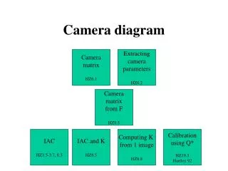
Camera diagram. Camera matrix HZ6.1. Extracting camera parameters HZ6.2. Camera matrix from F HZ9.5. IAC HZ3.5-3.7, 8.5. IAC and K HZ8.5. Computing K from 1 image HZ8.8. Calibration using Q* HZ19.3 Hartley 92. Camera terminology.


Camera diagram
E N D
Presentation Transcript
Camera diagram Camera matrix HZ6.1 Extracting camera parameters HZ6.2 Camera matrix from F HZ9.5 IAC HZ3.5-3.7, 8.5 IAC and K HZ8.5 Computing K from 1 image HZ8.8 Calibration using Q* HZ19.3 Hartley 92
Camera terminology • a camera is defined by an optical center c and an image plane • image plane (or focal plane) is at distance f from the camera center • f is called the focal length • camera center = optical center • principal axis = the line through camera center orthogonal to image plane • principal point = intersection of principal axis with image plane • an indication of the camera center in the image • principal plane = the plane through camera center parallel to image plane
Camera matrix Camera matrix HZ6.1 Extracting camera parameters HZ6.2 Camera matrix from F HZ9.5 IAC HZ3.5-3.7, 8.5 IAC and K HZ8.5 Computing K from 1 image HZ8.8 Calibration using Q* HZ19.3 Hartley 92
Encoding in a camera matrix • the act of imaging is encoded by the camera matrix P, which is 3x4: • x = point in image = 3-vector • X = point in 3-space being imaged = 4-vector • PX = x • in an early lecture, we saw that perspective projection is a linear operation in projective space, which allows this encoding • we will develop the camera matrix in stages, generalizing as we go
Camera matrix 1 • assumption set: • square pixels • origin of 3D world frame = camera center • z-axis of 3D world frame = principal axis • origin of 2D image space = principal point • P = diag(f,f,1)[I 0] • (X,Y,Z,1) (fX, fY, Z)
Camera matrix 2 (general image space) • remove assumption #4: origin of 2D image space is arbitrary, so principal point is (px,py) • Euclidean space: (X,Y,Z) (fX/Z + px, fY/Z + py) • projective space: (fX + Zpx, fY + Zpy, Z) • matrix: P = K[I 0] where K = (f 0 px; 0 f py; 0 0 1)
Camera matrix 3 (general world frame) • remove assumptions #2 and #3: origin and z-axis of the world frame are arbitrary, or equivalently, the world frame has no explicit connection to the camera • freeing the origin from the camera center involves a translation C • freeing the z-axis from the principal axis involves a rotation R • let X be a point in world frame coordinates and Xcam be the point in camera frame coordinates (with origin and z-axis aligned with camera): • Euclidean: Xcam = R(X-C) • projective: Xcam = [R –RC; 0 1] X • so imaging process is x = PXcam = K[I 0] Xcam = [K 0][R –RC; 0 1] X = [KR -KRC] X = KR[I –C] X • x = KR[I –C]X or P = KR[I –C] • HZ154-156 for last 3 slides
Camera matrix 4 (rectangular pixels) • remove assumption #1: pixels may no longer be square • cameras typically have non-square pixels • let mx = # of pixels / x-unit in image coordinates • let my = # of pixels / y-unit in image coordinates • e.g., mx = 1.333 and my = 1 if pixels are wider • XcamRect = diag (mx, my, 1) XcamSquare = diag(mx,my,1) [R –RC; 0 1] X • still write P = KR [I –C], but now the calibration matrix is • K = diag(mx,my,1) [f 0 px; 0 f py; 0 0 1] = [fmx 0 mxpx; 0 fmymypy; 0 0 1] • K is called the calibration matrix because it contains all of the internal camera parameters • we will be solving for K in the last stages as we solve for metric structure • K now has 10dof (encodes a CCD camera) • can also add a skew parameter s in k12 entry, yielding a finite projective camera • HZ156-7
Camera parameters Camera matrix HZ6.1 Extracting camera parameters HZ6.2 Camera matrix from F HZ9.5 IAC HZ3.5-3.7, 8.5 IAC and K HZ8.5 Computing K from 1 image HZ8.8 Calibration using Q* HZ19.3 Hartley 92
Extracting camera parameters from P • what do we want to know about a camera? • a camera is defined by its center (position) and image plane (part of orientation) • can compute image plane from center, principal plane, and focal length • can also compute image plane from center, principal axis, and focal length • all of these can be extracted from the camera matrix P • also important to know orientation of the camera • that is, the rotation from the world frame to the camera frame • gives orientation of image rectangle • therefore, want rotation matrix R (as in P = KR [I –C]) • the principal point is extractable from the camera center and image plane, but we can also find it directly from the camera matrix, if so desired
Camera center from P • let’s characterize finite cameras (with finite camera centers) • Fact: camera matrices of finite cameras = 3x4 matrices with nonsingular 3x3 left submatrix (nonsingular KR) • easy to see that KR is nonsingular for finite focal lengths • the camera center C (of a finite camera) is the null vector of camera matrix P • P is 3x4 with nonsingular 3x3 left submatrix, so has a 1D null space • proof: let C be null vector; all points on a line through C will project to the same point since P((1-t)C + tA) = PA; the only lines that map to a point are those through the camera center • another proof: the projection of C, PC, is undefined, which characterizes the camera center • C = (-M-1 p4 1) where p4 = last column of P and M = left 3x3 submatrix • recall that C in KR[I –C] was the camera center (in Euclidean space) • we want to extract –C from P • let P = KR [I –C’]; if C = (C’ 1), then PC = 0 • p4 = -KRC’ = -MC’ • exercise: where do you think camera center of infinite camera is? • infinite camera: center is defined by the null vector of M: C = (d, 0) where Md = 0 • M is singular in this case, so it does have a null vector • note that this is a point at infinity • HZ157-9
Exercise • before we talk about principal planes, we need a projective representation for the plane • What do you think it is? • Hint: it is the natural generalization of the projective representation of a line • Take 2 minutes.
Principal plane from P • a plane may be represented by ax+by+cz+d = 0; which is represented in projective space by the 4-vector (a,b,c,d) • points on the principal plane are distinguished as the only ones that are mapped to infinity by the camera • that is, PX is an ideal point with x3=0 • that is, P3T X = 0, where P3T is the 3rd row of P • that is, the principal plane is P3T • note that this plane does contain the camera center, as it should • PC = 0 P3T C = 0 • HZ160
Focal length and R from P • finding focal length reduces to finding the calibration matrix K • focal length is encoded on the diagonal of K: (fmx fmy 1) • where (mx, my) is the pixel’s aspect ratio • recall that K and R are embedded in the front of the camera matrix P • P = KR [I –C] • we simply need to factor • let M = KR = left 3x3 submatrix of P • K is upper triangular, R is orthogonal • recall QR decomposition from numerical computing • A = QR where Q is orthogonal (e.g., product of Householders) and R is upper triangular • perfect, except wrong order • RQ decomposition is analogous • HZ157
RQ decomposition • A = RQ, where R = upper triangular, Q = orthogonal • we want to reduce A to upper triangular: A R • need to zero a21, a31 and a32 • use 3 Givens rotations • A G1 G2 G3 = R • so A = R (G1 G2 G3)^t • Q = (G1 G2 G3)^t • zero carefully to avoid contamination • zero a32 with x-rotation G1, then a31 with y-rotation G2, then a21 with z-rotation G3 • i.e., reverse order of A entries • Qy leaves 2nd column alone (so a32 remains zero) • Qz creates new 1st and 2nd columns from linear combinations of old 1st and 2nd columns, so 3rd row remains zeroed (cute!) • Q represents a rotation, which can be encoded by roll/pitch/yaw • angles associated with Gi are these 3 angles of roll/pitch/yaw (also called Euler angles) • HZ579
Solving for Euler angle • the first Givens rotation zeroes a32 • let G1 = (1 0 0; 0 c –s; 0 s c) rotate about x • a32 element of AG1 = c*a32 + s*a33 • a32’ = 0 c:s = -a33 : a32 c = k(-a33); s = k(a32); c2 + s2 = 1 k2(a332 + a322) = 1 k = sqrt(a322 + a332) • we now know G1 • solve for G2 and G3 analogously
Exercise • before we talk about principal axis, we need to recall a basic fact about the normal of a plane • what is the normal of the plane ax+by+cz+d=0? why? • take 2 minutes as a group
Principal axis from P • the normal of a plane ax+by+cz+d = 0 is (a,b,c) • why? (X-P).N = 0 becomes X.N – P.N = 0 • the principal axis is a normal of the principal plane • recall: the principal plane is the third row of P (we called it P3T) • Exercise: what is the normal of the principal plane? • let M3T = third row of M • normal of the principal plane = M3 • so principal axis direction = M3 • which direction, M3 or –M3, points towards front of camera? • answer: det(M) M3 • det(M) protects it against sign changes • principal axis = det(M) M3
Principal point from P • the principal point is less important, but let’s look at it anyway • we could find the principal point by intersecting the line normal to the principal plane and through the camera center with the image plane • but this does not relate back directly to the camera matrix • let’s relate directly to P • principal point = image of the point at infinity in the direction of the principal plane’s normal • the point at infinity in this direction is (M3 0) • P (M3 0) = MM3 • principal point = MM3, where M3T is the third row of M • HZ160-161