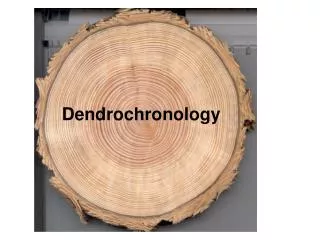
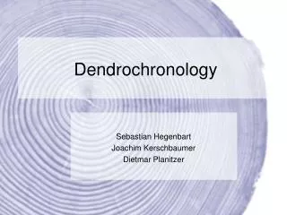
Dendrochronology

1. Dendrochronology Sebastian Hegenbart Joachim Kerschbaumer Dietmar Planitzer

2. Introduction • Dendrochronology • Motivation and target • Preprocessing • Center point detection • Generating profiles and analysis

3. Dendrochronology • Tree-ring dating • Analysis of tree-ring growth patterns • Annual rings of different properties depending on weather, rain, temperatur, etc. in different years • Used to date pieces of wood and when they were felled.

4. Motivation and target • CT images of timber samples as input • Preprocessing for image enhancement • Skeletonizing • Detection of center point • Counting and analyzing annual rings

5. Implementation • Three major steps: • Preprocessing • Finding the Center • Generating Profiles

6. Preprocessing • Remove noise with a 3x3 Gauss filter • Local contrast enhancement • Isolate rings with a 5x5 Mexican Hat • Convert to binary with 50% threshold • Gabor Filtering • Skeletonization • Cleaning

7. Input Image

8. Local Contrast Enhancement • Adaptive algorithm from Yu & Bajaj • Operates on a 5x5 window • Computes local pixel min/max/avg values • Applies a stretching window • Applies an adaptive transfer function

9. Local Contrast Enhancement

10. Mexican Hat

11. Gabor Transformation • Dennis Gábor (1946) • Windowed Fourier Transform • Gaussian function as windowing function

12. Gabor Transformation contd. • Gabor Transformation : • Orientation  • Frequency f • Sigma (standard deviation of gaussian distribution) • Selection of sigma involves a tradeoff • Larger values: more robust to noise but more likely to create spurious rings • Smaller values:less likely produce spurious rings but less effective in removing noise

13. Gabor Transform contd. • Timber CT images: • Sigma = 4 • 3 different frequencies for detecting large,medium and small rings • Gabor Filter:

14. Gabor Transform contd. • Gabor filter applied to wood image

15. Gabor Implementation • Creation of gabor filters with different frequencies and orientations • Convolution operations with filters • Rotation from 0 to 180 degrees • Assemble output images

16. Gabor Transform

17. Gabor Transform

18. Skeletonization I • Set white pixel if 4 conditions are fullfilled • Condition 1: pixel p[x,y] must presently be black. If the pixel is already white, no action needs to be taken • Condition 2: At least one of the pixels close neighbours must be white • Condition 3: the pixel must have more than one black neighbour. If it has only one, it must be the end of a line, and therefore shouldnt be removed. • Condition 4: a pixel cannot be removed if it results in its neighbours being disconnected.

19. Skeletonization II • Thinning algorithm from Zhang & Suen • With improvements from Holt and Stentiford • Must guarantee that a line is exactly 1 pixel thick • Stair case removal

20. Skeletonization

21. Twig Removal • Sometimes short curves (twigs) extend out of year rings • Those are artifacts of the scanning or skeletonization process • Danger of misinterpreting them as year rings • Consequently, they must be removed

22. Twig Removal • Scan the image looking for T-junctions • Compute the length of all curves connected to a T-junction • A curve is a twig if its length is less a threshold • Remove the pixel which connects a twig to a year ring

23. Image Cleaner • Removes short curves from the image • Those are often artifacts of the scanning process • All curves with length less a threshold are removed • This includes twigs

24. Image Cleaner • Scan the image looking for curves • Trace the curve and measure its length • If the length is less a threshold, then remove it

25. Cleaned Image

26. Center point localization • Hough-Transform • Approximation by Curvature • Gradient Accumulation • Poincaré Index

27. Center point definition

28. Hough-Transform • Feature extraction technique used in digital image processing. • Used with binary images after edge detection. • The pixel space is transformed into parameter space by accumulation of all possible parameters (for a certain parameterized curve) for every edge pixel inside the pixel space. • 3-Dimensional parameter space for circles.

29. Hough-Transform Figure 1. Successfull Detection Figure 2. Failed Detection

30. Hough-Transform • Summary: • Complexity O(n³) • Brute Force • No perfect circles • Sensitive to noise • Conclusion: • Not suited to find center in pure form

31. Approximating center by segment curvature. • Idea: Curvature increases heading to the center. • Curvature = 1 / Radius • Problems: • Need a way to calculate radius for a given Segment.

32. Approximating center by segment curvature. • Find a connected segment of pixels and follow it. • Calculate s as the euclid distance between start and end point of the circular arc. • Calculate normal Vector of AB and follow it to the next black pixel. • Validate if the pixel is part of the arc segment by following the segment to either A and B. • Calculate h as the euclid distance between the point of intersection and the center of AB. Figure 4. Calculation of h and s.

33. Approximating center by segment curvature. • Tresholding on curvature to identify segments close to the center. • Use statistical methods to throw away stray „red“ segments. • Average segment‘s center points to estimate center. • Use hough transform on a 64 x 64 pixel window around estimated center to find the real center point. Figure 5. Successfull Detection

34. Approximating center by segment curvature. • Summary: • works best with circular images (can use hough) • estimating center works best with a limited number of „red“ segments • twigs and distortions can fake a high curvature • requires connected segments • Conclusion: • works best combined with Hough-Transform • works best with cirular images • sensitive to twigs and cuts Figure 6. Failed Detection

35. Gradient Accumulation • Idea: Gradients of segments point toward the center. • Problems: • Need a way to calculate the gradient for any given segment. • Need a way to evaluate the gradient‘s direction.

36. Gradient Accumulation • Gradient Calculation: • Compute Gradients either by derivative using Sobel/Prewitt Masks. (see Poincaré) • Follow line segments, identify tangent and calculate gradient from tangent. Figure 7. Successfull Detection

37. Gradient Accumulation • Evaluating Gradient Direction: • Follow Gradient Orientation in either direction and accumulate each hit pixel in an array. • Use Maximum value inside the accumulator to identify center. • Alternatively calculate barycenter of accumulator or use box filtering. Figure 8. Filled Accumulator

38. Gradient Accumulation • Summary: • Simple and fast • Insensitive to twigs and distortions • Finding the center inside the accumulator can be tricky • Works well with both kind of images • Conclusion: • Probably the best technique

39. Poincaré Index • Used in fingerprint images to identify singularities. • Based on an Orientation image. • Idea: The total rotation of the vectors along a closed curve is 360° • Problems: • How to calculate the orientation image ? • How to average angles ?

40. PoincaréIndex • Generating the orientation image: • use Sobel Masks to calculate the derivatives in x and y Gx Gy • Problems with derivatives: • The derivative of a vertical line in x is 0 and vice versa • Also the derivative of a line with 45° of angle is 0

41. Poincaré Index • Solution: (Let‘s call the derivatives in x = Gx and in y = Gy ) • If Gx = 0, assume a horizontal orientation (i.e. 0°) • If Gy = 0, assume a vertical orientation (i.e. 90°) • If both Gx and Gy = 0, throw the pixel away • Else calculate the orientation as:

42. Poincaré Index • Averaging angles: • A single pixel orientation is not very strong, a way is needed to average pixel orientations over a window. • Angles can not be averaged arithmetically (e.g.: the angle between 175° and 5° is 0 °) • A solution to this problem is splitting the orientation into it‘s sine and cosine parts and then calculate their arithmetic mean.

43. Poincaré Index Averaging angles inside a window: (note the division to account for 0° segments)

44. Poincaré Index • Once the orientation field is generated the poincaré index can be computed. • Care has to be taken to respect the orientation. • The Poincaré index then computes as: Figure 9. Poincaré Index (source: Handbook of Fingerprint Recognition) Figure 10. Orientation Field

45. Poincaré Index Figure 10. Failed Detection Figure 11. Successfull Detection

46. Poincaré Index • Summary: • Tricky to implement • Many practical problems • Center point accuracy depends on the size of the averaging window • Orientation accuracy depends on the size of the averaging window • Conclusion: • probably better than curvature approximation • does not work with images without a closed curve • can be modified to find -180° and 180° singularities

47. Profile Generation • Trunk is scanned from the outside to the inside • Strictly along a straight line • Generating multiple profiles by going counter clockwise around the trunk • Only accept profile if the difference between year rings is less a threshold

48. Profile Generation • Scanning year rings along a straight line using the Bresenham algorithm • Scan window must be 2x1, otherwise a year ring might be missed • Profile records the distance between year rings • Profile data is normalized in the end

49. Application

50. Application