8. MODELING TRACE METALS
8. MODELING TRACE METALS. Art is the lie that helps us to see the truth. - Pablo Picasso. 8.1 INTRODUCTION.


8. MODELING TRACE METALS
E N D
Presentation Transcript
8. MODELING TRACE METALS Art is the lie that helps us to see the truth. - Pablo Picasso
8.1 INTRODUCTION • Modeling is a little like art in the words of Pablo Picasso. It is never completely realistic; it is never the truth. But it contains enough of the truth, hopefully, and enough realism to gain understanding about environmental systems. • Improvements in analytical quantitation have affected markedly the basis for governmental regulation of trace metals and increased the importance of mathematical modeling. • Figure 8.1 was compiled from manufacturers‘ literature on detection limits for lead in water samples. As we changed from using wet chemical techniques for lead analysis (1950-l960), to flame atomic absorption (1960-1975), to graphite furnace atomic absorption (1975-l990), to inductively coupled plasma mass spectrometry with preconcentration (1985-present), the limit of detection has improved from approximately 10-5 (10 mg L-1) to 10-l2 (1.0 ng L-1). • In some cases, water quality standards have become more stringent when there are demonstrated effects at low concentrations. • Some perspective on Figure 8.1 is provided by Table 1.3. Drinking water standards are given in Table 8.1 for metals and inorganic chemicals.
Figure 8.1 Analytical limits of detection for lead in environmental water samples since 1960 Table 8.1 Maximum contaminant level (MCL) drinking water standards for inorganic chemicals and metals (mg L-1 except as noted)
"Heavy metals" usually refer to those metals between atomic number 21 (scandium) and atomic number 84 (polonium), which occur either naturally or from anthropogenic sources in natural waters. These metals are sometimes toxic to aquatic organisms depending on their concentration and chemical speciation. • Heavy metals differ from xenobiotic organic pollutants in that they frequently have natural background sources from dissolution of rocks and minerals. The mass of total meta1 is conservative in the environment; although the pollutant may change its chemical speciation, the total remains constant. • Heavy metals are a serious pollution problem when their concentration exceeds water quality standards. Thus waste load allocations are needed to determine the permissible discharges of heavy metals by industries and municipalities. • In addition, volatile metals (Cd, Zn, Hg, Pb) are emitted from stack gases, and fly ashes contain significant concentrations of As, Se, and Cr, all of which can be deposited to water and soil by dry deposition.
8.1.1 Hydrolysis of Metals • All metal cations in water are hydrated, that is, they form aquo complexes with H2O. • The number of water molecules that are coordinated around a water is usually four or six. We refer to the metal ion with coordinated water molecules as the “free aquo metal ion”. • The analogous situation is when one writes H+ rather than H3O+ for a proton in water; the coordination number is one for a proton. • The acidity of H2O molecules in the hydration shell of a metal ion is much larger than the bulk water due to the repulsion of protons in H2O molecules by the + charge of the metal ion. • Trivalent aluminum ions (monomers) coordinate six waters. Al3+ is quite acidic, (1) • because the charge to ionic radius ratio of A13+ is large. Al3+· 6 H2O can also be written as Al(H2O)3+6
The maximum coordination number or metal cations for ligands in solution is usually two times its charge. Metal cations coordinate 2, 4, 6, or sometimes 8 ligands. Copper (II) is an example of a metal cation with a maximum coordination number of 4. (2) (3) • Metal ions can hydrolyze in solution, demonstrating their acidic property. This discussion follows that of Stumm and Morgan. (4) • Equation (4) can be written more succinctly below. (5) • Kl is the equilibrium constant, the first acidity constant. • If hydrolysis leads to supersaturated conditions or metal ions with respect to their oxide or hydroxide precipitates, thus: (6) • Formation or precipitates can be considered as the final stage of polynuclear complex formation: (7)
8.1.2 Chemical Speciation • Speciation of metals determines their toxicity. Often, free aguo metal ions are toxic to aquatic biota and the complexed metal ion is not. Chemical speciation also affects the relative degree of adsorption or binding to particles in natural waters, which affects its fate (sedimentation, precipitation, volatilization) and toxicity. • Figure 8.2 is a periodic chart that has been abbreviated to emphasize the chemistry of metals into two categories of behavior: A-cations (hard) or B-cations (soft). • The classification of A- and B-type metal cations is determined by the number of electrons in the outer d orbital. Type-A metal cations have an inert gas type of arrangement with no electrons (or few electrons) in the d orbital, corresponding to "hard sphere“ cations. • Type-A metals form complexes with F- and oxygen donor atoms in ligands such as OH-, CO32-, and HCO32-. They coordinate more strongly with H2O molecules than NH3 or CN-. • Type-B metals (e.g., Ag+, Au+, Hg2+, Cu+, Cd2+) have many electrons in the outer d orbital. They are not spherical, and their electron cloud is easily deformed by ligand fields.
Transition metal cations are in-between Type A and Type B on the periodic chart (Figure 8.2). They have some of the properties of both hard and soft metal cations, and they employ 1-9 d electrons in their outer orbital. • A qualitative generalization of the stability of complexes formed by the transition metal ions is the Irving-Williams series: (8) • These transition metal cations show mostly Type-A (hard sphere) properties. Zinc (II) is variable in the strength of its complexes; it forms weaker complexes than copper (II), but stronger complexes than several of the others in the transition series. • Table 8.2 gives the typical species of metal ions in fresh water and seawater. This is a generalization because the species may change with the chemistry of an individual natural water. • Table 8.2 is applicable to aerobic waters-anaerobic systems would have large HS- concentrations that would likely precipitate Hg(II), Cd(II), and several other Type-B metal cations.
Figure 8.2 Partial periodic table showing hard (A-type) metal cations and soft (B-type) metal cations
Table 8.2 Major species of metal cations in aerobic fresh water and seawater
8.1.3 Dissolved Versus Particulate Metals • Heavy metals that have a tendency to form strong complexes in solution also have a tendency to fem surface complexes with those same ligands on particles. Difficulty arises because chemical equilibrium models must distinguish between what is actually dissolved in water versus that which is adsorbed. Analytical chemists have devised an operational definition of "dissolved constituents" as all those which pass a 0.457 µm membrane filter. • Windom et al. and Cohen have demonstrated that filtered samples can become easily contaminated in the filtration process. As per Horowitz, there are two philosophies for processing a filtered sample for quantitation of dissolved trace elements: • (1) treat the colloidally associated trace elements as contaminants and attempt to exclude them from the sample as much as possible, or • (2) process the sample in such a way that most colloids will pass the filter (large particles will not) and try to standardize the technique so that results are operationally comparable.
Shiller and Taylor and Buffle have proposed ultrafiltration, sequential flow fractionation, or exhaustive filtration as methods to approach the goal of excluding colloidally associated metals from the water sample entirely. • Flegal and Coale were among the first to report that previous trace metal data sets suffered from serious contamination problems. The modeler needs to under stand how water samples were obtained because it can affect results when simulating trace metals concentrations in the nanogram per liter range, especially. • According to Benoit, ultraclean procedures have three guiding principles: - (1) samples contact only surfaces consisting of materials that are low in metals and that have been extensively acid-cleaned in a filtered air environment; - (2) samples are collected and transported taking extraordinary care to avoid contamination from field personnel or their gear; - (3) all other sample handling steps take place in a filtered air environment and using ultra-pure reagents. • The "sediment-dependent" partition coefficient for metals (Kd) is an artifact, to large extent, of the filtration procedure in which colloid-associated trace metals pass the filter and are considered "dissolved constituents”.
8.2 MASS BAIANCE AND WASTE LOAD ALLOCATION FOR RIVERS 8.2.1 Open-Channel Hydraulics • A one-dimensional model is the St. Venant equations for nonsteady, open-channel flow. We must know where the water is moving before we can model the trace metal constituents. (9) (10) • where Q = discharge, L3T-1 t = time, T z = absolute elevation of water level above sea level, L A = total area of cross section, L2 b = width at water level, L g = gravitational acceleration, LT-2 x = longitudinal distance, L qi = lateral inflow per unit length of river, L2T-1 Sf = the friction slope: (11)
Only a few numerical codes that are available solve the fully dynamic open-channel flow equations. It requires detailed cross-sectional area/stage relationships, stage/discharge relationships, and stage and discharge measurements with time. • Trace metals are often associated with bed sediments, and sediment transport is very nonlinear. Bed sediment is scoured during flood events when critical shear stresses at the bed-water interfaces are exceeded. • Necessary to solve the fully dynamic St. Venant equations. • Equations (9) and (10) can be simplified: • (1) lateral inflow qi can be neglected and accounted for at the beginning of each stream segment; • (2) the river can be segmented into reaches where Q(x) is approximately constant within each segment; • (3) the river can be segmented into reaches where A(x) is approximately constant within each segment. • If Q and A can be approximated as constants in (x, t), then the velocity is constant and the problem reduces to one or steady flow.
8.2.2 Mass Balance Equation • Figure 8.3: a schematic of trace metal transport in a river. Metals can be in the particulate-adsorbed or dissolved phases in the sediment or overlying water column. Interchange between sorbed metal ions and aqueous metal ions occurs via adsorption/desorption mechanisms. • Bed sediment can be scoured and can enter the water column, and suspended solids can undergo sedimentation and be deposited on the bed. Metal ions in pore water of the sediment can diffuse to the overlying water column and vice versa, depending on the concentration driving force. • Under steady flow conditions (dQ/dt = 0), we can consider the time-variable concentration of metal ions in sediment and overlying water. We will assume that adsorption and desorption processes are fast relative to transport processes and that the suspended solids concentration is constant within the river segment. • Sorption kinetics are typically complete within 1 hour, which is fast compared to transport processes, except perhaps during high-flow events. Suspended solids concentrations can be assumed as constant within a segment under steady flow conditions.
The modeling approach is to couple a chemical equilibrium model with the mass balance equations for total metal concentration in the water column. • In this way, we do not have to write a mass balance equation for every chemical species (which is impractical). The approach assumes that chemical equilibrium among metal species in solution and between phases is valid. • Acid-base reactions and complexation reactions are fast (on the order of minutes to microseconds). Precipitation and dissolution reactions can be slow; if this is the case, the chemical equilibrium submodel will flag the relevant solid phase reaction (provided that the user has anticipated the possibility). • Redox reactions can also be slow. The modeler must have some knowledge of aquatic chemistry in order to make an intelligent choice of chemical species in the equilibrium model. • Assuming local equilibrium for sorption, we may write the mass balance equations similarly to those given in Chapter 7 for toxic organic chemicals in a river. The only difference is that metals do not degrade-they may undergo chemical reactions or biologically mediated redox transformations, but the tota1 amount of metal remains unchanged.
If chemical equilibrium does not apply, each chemical species of concern must be simulated with its own mass balance equation. • An example would be the methylation and dimethylation of Hg and Hg0 volatilization, which are relatively slow processes, and chemical equilibrium would not apply. (12) (13)
Where CT = total whole water (unfiltered) concentration in the water column, M L-3 t = time, T A = cross sectional area, L2 Q = flowrate, L3T-1 x = longitudinal distance, L E = longitudinal dispersion coefficient, L2T-1 ks = sedimentation rate constant, T-1 fp,w = particulate adsorbed fraction in the water column, dimensionless fd,w = dissolved chemical fraction in the water column, dimensionless Kp,b = sediment-water distribution coefficient in the bed, L3M-1 r = adsorbed chemical in bed sediment, MM-1 kL = mass transfer coefficient between bed sediment and water column, LT-1 h = depth of the water column (stage), L α = scour coefficient of bed sediment into overlying water, T-1 Sb = bed sediment so1ids Concentration, ML-3 bed volume γ = ratio of water depth to active bed sediment layer, dimensionless d = depth of active bed sediment, L
The model is similar to that depicted in Figure 8.3 except that we assume instantaneous sorption equilibrium in the water column and sediment between the adsorbed and dissolved chemical phases. • The first two terms of equation (12) are for advective and dispersive transport for the case of variable Q, E, and A with distance. • The last term in equations (12) and (13) accounts for scour of particulate adsorbed material from the bed sediment to the overlying water using a first-order coefficient for scour, α, that would depend on flow and sediment properties. • Equations (12) and (13) are a set of partial differential equations that can be solved by the method of characteristics or operator splitting methods. • This set of two equations is very powerful because it can be used to model situations when the bed is contaminated and diffusing into the overlying water or when there are point source discharges that adsorb and settle out of the water column to the bed.
Figure 8.3 Schematic model of metal transport in a stream or river showing suspended and bed load transport of dissolved and adsorbed particulate material.
Local equilibrium was assumed in equations (12) and (13) for adsorption and desorption. If a simple equilibrium distribution coefficient is applicable, one can substitute for the fraction or chemical that is dissolved and particulate according to the following relationships: • Where fd,w = fraction dissolved in the water column fp,w = fraction in particulate adsorbed form in the water column Kp,w = distribution coefficient in the water, L kg-1 Sw = suspended so] ids concentration, kg L-1 • Alternatively, one can use a chemical equilibrium submodel to compute Kp,b,fd,w and fp,w in the water and sediment. In this case, several options are available including Langmuir sorption, diffuse double-layer model, constant capacitance model, or triple-layer model.
8.2.3 Waste Load Allocation • Point source discharges that continue for a long period will eventually come to steady state with respect to river water quality concentrations. The steady state will be perturbed by rainfall runoff discharge events, but the river may tend toward an "average condition”. • Under steady-state conditions (∂CT/∂t = 0 and ∂r/∂t = 0), equations (12) and (13) reduce to the following: (14) • For large rivers, after an initial mixing period, dispersion can be estimated by Fischer's equation: (15), (16) • where g is the gravitational constant (LT-2), h is the mean depth (L), and S is the energy slope of the channel (LL-1).
A mixing zone in the river is allowed in the vicinity of the wastewater discharge where locally high concentrations may exist before there is adequate time for mixing across the channel and with depth. • The mixing zone can be estimated from the empirical equation (17): (17) • where Xℓ = mixing length for a side bank discharge, ft B = river width, ft Ey = lateral dispersion coefficient, ft2 s-1 = єhu* є = proportionality coefficient = 0.3 - 1.0 u* = shear velocity as defined in equation (16), ft s-1 h = mean depth, ft • The most basic waste load allocation is a simple dilution calculation assuming complete mixing or the waste discharge with the upstream metals concentration. One assumes that the total metal concentration (dissolved plus particulate adsorbed concentrations) are bioavailable to biota as a worst case condition.
At the next level or complexity, the waste load allocation may become a probalistic calculation using Monte Carlo analysis. • Using the following equation: • Where CT = total metals concentration, ML-3 Qu = upstream flowrate, L3T-1 Cu = upstream metals concentration, ML-3 Qw = wastewater discharge flowrate, L3T-1 Cw = wastewater metals concentration, ML-3 • The steps in the procedure include estimating a frequency histogram (probability density function) for each of the four model parameters Qu,Cu,Qw and Cw. • Usually, normal or lognormal distributions are assumed or estimated from field data. A mean and a standard deviation are specified.
A more detailed waste load allocation was prepared for the Deep River in Forsyth County, North Carolina. A steady-state mass balance equation was used that neglected longitudinal dispersion and scour. (18) • Equation (18) was coupled with a MINTEQ chemical equilibrium model to determine chemical speciation of dissolved metal cations. • Figure 8.4 is the result of the waste load allocation. Steps in the procedure were the following: • 1. Select critical conditions when concentrations and/or toxicity are expected to be greatest. Usually 7-day, 1-in- l0-year low-flow periods are assumed. • 2. Develop an effluent discharge database. If measured flow and concentration data are not available for each discharge, the maximum permitted values are usually assumed, or some fraction thereof.
3.Obtain stream survey concentration data during critical conditions. Suspended solids, bed sediment, and filtered and unfiltered water samples should be analyzed for each trace metal of concern. Dye studies for time of travel, gage station flow data (stage-discharge), and cross-sectional areas of the river reach should be obtained. Measurement of nonpoint source loads should also be accomplished at this time. • 4. Perform model simulations. First, calibrate the model by using the effluent discharge database and the stream survey results. Adjustable parameters include ks and kL. All other parameters and coefficients should have been measured. ks and kL should be varied within a reasonable range of reported literature values. • 5. Determine how much the measured trace metal concentrations exceed the water quality standard. (If they do not exceed the standard, there is no need for a waste load allocation.) Reduce the effluent discharges proportionally until the entire concentration profile is within acceptable limits.
Figure 8.4 Waste load allocation for copper in the Deep River, North Carolina. Total dissolved copper concentrations in field samples and model simulation are shown. The water quality standard is 20 µg L-1.
5.3 COMPLFX FORMATION AND SOLUBILITY 8.3.1 Formation Constants • Complexation or free aquo metal ions in solution can affect toxicity markedly. Stability constants are equilibrium values for the formation of complexes in water. • They can be expressed as either stepwise constants or overall stability constants. • Stepwise constants are given by equations (19) to (21) as general reactions, neglecting charge. (19) (20) (21)
Overall stability constants are reactions written in terms of the free aquo metal ion as reactant: (22) (23) • The product of the stepwise formation constants gives the overall stability constant: (24) • For polynuclear complexes, the overall stability constant is used, and it reflects the composition of the complex in its subscript. An example would be Fe2(OH)24+ (25) (26)
Table 8.3 Logarithm of Overall Stability Constants for Formation of Complexes and Solid from Metals and Ligands at 25 °C and I = 0.0 M
Table 8.3 is adapted from Morel and Hering, and it provides some common overall stability constants and solubility constants for 19 metals and 10 ligands. • Note that the values are given as log β values for the formation constants. (27) • The stability and solubility constants are given at 25 °C and zero ionic strength (infinite dilution). At low ionic strengths, the constants may be used with concentrations rather than the activities indicated by the brackets in equations (19)-(27). • Complexation reactions are normally fast relative to transport reactions, but precipitation and dissolution reactions can be quite slow (mass transfer or kinetic limitations). • Under anaerobic conditions, sulfide is generated; it is a microbially mediated process of sulfate reduction in sediments and groundwater.
8.3.2 Complexation by Humic Substances • Humic substances comprise most naturally occurring organic matter (NOM) in soils, surface waters, and groundwater. They are the decomposition products of plant tissue by microbes. Humic substances are separated from a water sample by adjusting the pH to 2.0 and capturing the humic materials on an XAD-8 resin; subsequent elution in dilute NaOH is used to recover the humic substances from the resin. • In nature, soils are leached by precipitation, and runoff carries a certain amount of humic and fulvic compounds into the water. (28) • The term fulvic acids (FA) refers to a mixture of natural organics with MW ≈ 200-5000, the fraction that is soluble in acid at pH 2 and also soluble in alcohol. The median molecular weight of FA is ~500 Daltons. • The fulvic fraction (FF) includes carbohydrates, fulvic acids, and polysaccharides. (29)
Table 8.4 is a summary of metal-fulvic acid (M-FA) complexation constants. • One approach is to use conditional stability constants (such as Table 8.4) for the natural water that is being modeled (30) • where cK is the conditional stability constant at a specified pH, ionic strength, and chemical composition. One does not always know the stoichiometry of the reaction in natural waters, whether 1:1 complexes or 1:2 complexes (M/FA) are formed, for example. • Equation (30) is simply a lumped-parameter conditional stability constant, but it does allow intercomparisons of the relative importance of complexation among different metal ions and DOC at specified conditions. • The conditional complexation constant (stability constant) should be measured for each site. Total dissolved concentrations of metals (including M-FA) are measured using atomic absorption spectroscopy or inductively coupled plasma emission spectroscopy, and the aquo free metal ion is measured by ISEs or ASV.
Table 8.4 Freshwater conditional stability constants for formation of M-FA complexes (roughly in order of binding strength)
Conditional stability constants for metal-fulvic acid complexes vary in natural waters because: • There are a range of affinities for metal ions and protons in natural organic matter resulting in a range of stability constants and acidity constants. • Conformational changes and changes in binding strength of M-FA complexes in natural organic matter result from electrostatic charges (ionic strength), differential and competitive cation binding, and, most of all, pH variations in water. • The stability constants given in Table 8.5 vary markedly with pH. • The total number of metal-titrateable groups is in the range of 0.1 - 5 meq per gram of carbon, DOC complexation capacity. Complexation of metals fulvic acid is most significant for those ions that are appreciably complexed with CO32- and OH- (functional groups like those contained in fulvic acid that contains carboxylic acids and catechol with adjacent - OH sites). These include mercury, copper, and lead.
Using only one conditional stability constant for Cu-FA, Figure 8.6 demonstrates the importance of including organics complexation in chemical equilibrium modeling for metals. • The MINTEQ chemical equilibrium program was used lo solve the equilibrium problem, and the distribution diagrams for chemical speciation are given in Figure 8.6. MINTEQ was used to find the percentage of each species of Cu(II) at pH increments of 0.5 units. • Results in Figure 8.6a show that at the pH of the sample (pH 6.1) and below, the copper is almost totally as free aquo metal ion (hypothetically, in the absence of FA complexing agent). • Figure 8.6b shows that, in reality, almost all of the dissolved Cu(II) is present as the Cu-FA complex. Only 2% of the copper is present as the free aquo metal ion (~ 0.12 µg L-1 or 1.9 × 10⁻⁹ M). This is 100 times below the chronic threshold water quality criterion (based on toxicity) of 12 µg L-1. • In Figure 8.7a, assuming an absence of FA complexing agent, the free aquo cadmium concentration would be nearly 5 µg L-1 at pH 6.1. Thus the free aquo Cd2+ concentration is modeled to be 4.3 µg L-1 (3.9 × 10⁻⁸ M) with fulvic acid present, about 87% of the total dissolved cadmium concentration at pH 6.1 (Figure 8.7b.).
Figure 8.6 • Equilibrium chemical speciation of Cu(II) in Filson Creek, Minnesota, without consideration of complexation by dissolved organic carbon (fulvic acid). • Equilibrium chemical speciation of Cu(II) in Filson Creek, Minnesota, with copper-fulvic acid formation constant of log K = 6.2.
Figure 8.7 • Equilibrium chemical speciation of Cd(II) in Filson Creek, Minnesota, without consideration of complexation by dissolved organic carbon (fulvic acid). • Equilibrium chemical speciation of Cd(II) in Filson Creek, Minnesota, with cadmium-fulvic acid formation constant of log K = 3.5.
Example 8.2 Lead Chemical Speciation • A chemical equilibrium program with a built-in database can be used to model the chemical speciation for Pb in natural waters. Lake Hilderbrand, Wisconsin, is a small seepage lake in northern Wisconsin with some drainage from a bog. It receives acid deposition from air emissions in the Midwest, and its chemistry reflects acid precipitation, weathering/ion exchange with sediments, heavy metals deposition, and fulvic acids. • It was probably never an alkaline lake because much of its water comes directly onto the surface of the lake via precipitation and from drainage or bogs; the current pH is 5.38. It has 12.0 units of color (Pt-Co wits), an we can assume a FA concentration of 2.9 × 10⁻⁵ M. The log cK for Pb-FA in the system is in the range of 4-5. • Use a chemical equilibrium model such as MINTEQA2 to solve for all the Pb species in solution from pH 4 to 8 with increments of 0.5 units. The temperature of the sample was 13.7 °C. • Its ion chemistry (in mg L-1) was the following: Ca+2 = 1.37, Na+ = 0.21, Mg2+ = 0.31, K+ = 0.64, ANC (titration alkalinity as CaC03) = 0.03, SO42- = 5.25, Cl- = 0.38, Cd(II) = 0.000037, and Pb(II) = 0.00035 mg L-1. Is the Pb(II) expected to be present as the free aquo metal ion?
Solution: All the ions must be converted to mol L-1 concentration units. The ion balance should be checked; the sum of the cations minus the anions should be within 5% of the sum of the anions. At pH 5.38 some of the FA is anionic (fulvate), so it might need to be included as an anion in the charge balance. In this case, there is a good charge balance so the fulvic acid either • (1) has an acidity constant near the pH of the solution and it does not contribute much to the charge, and/or • (2) a portion of the Ca2+ is actually complexed by FA-, which fortuitously causes the calculated ∑(+) charges to be nearly equal to the ∑(-) charges. • The ion balance checks to within 2.4%.
At high pH we expect PbC03(aq) and PbOH+; at low pH we expect Pb2+ and possibly Pb-FA. • The acidity constant for HFA is log K = -4.8. • We neglect the complex of PbSO40 because the stability constant is rather small (Table 8.3). As we increase pH from 4 to 8, we can assume an open or a closed system with respect to CO2(g). In this case, a closed system was assumed. • Results for three different cases are given in Figure 8.8. The model is quite sensitive to the log cK that is assumed for the Pb-FA complex. Given a log cK = 5.0, most of the total lead that is present in solution is complexed with fulvic acid at pH 5.38. • Schnitzer and Skinner suggest an even stronger Pb-FA complex at pH 5 with log cK = 6.13 in soil water. Most of the Pb(II) is apparently complexed with fulvate at pH 5.38 in Lake Hilderbrand. It is not considered toxic; the chronic water quality criterion for fresh water is 3.2 µg L-1.
Figure 8.8 Lead speciation in Lake Hilderbrand, Wisconsin. (a) Without consideration of Pb-FA complexation. (b) With Pb-FA complexation, log K = 4. (c) With Pb-FA complexation, log K = 5
Example 8.2 brings up an important model limitation or fulvic acid binding for metal ions in natural waters. It is not clear how much competition exists among divalent cations. For example, the reaction between Ca-FA and Pb2+ in solution is certainly less favorable thermodynamically than FA with Pb2+. • These competition reactions (ligand exchange) are generally not considered in chemical equilibrium modeling. (31) • The log cK for Al-FA is approximately 5.0 (quite a strong complex), and this competition was not considered in Example 8.2. Also, the affinity of Fe(III) for FA is almost equal to that of Pb-FA. • Figure 8.9 shows the nature of those binding sites where adjacent carboxylic acid and phenolic groups are hydrogen bonded to form a polymeric structure with considerable stability. Figure 8.9 Typical structure of dissolved organic matter in natural waters with hydrogen bonding and bridging among functional groups that also make binding sites for metals.
8.4SURFACE COMPLEXATION/ADSORPTION 8.4.1 Particle-Metal Interactions • In addition to aqueous phase complexation by inorganic and organic ligands, meta1 ions can form surface complexes with particles in natural waters. This phenomenon is variously named in scientific literature as surface complexation ion exchange, adsorption, metal-particle binding, and metals scavenging by particles. • Particles in natural water are many and varied, including hydrous oxides, clay particles, organic detritus, and microorganisms. They range a wide gamut of sizes (Figure 8.10). • Particles provide surfaces for complexation of metal ions, acid-base reactions, and anion sorption. • where SOH represents hydrous oxide surface sites, M2+ is the metal ion, and A2- is the anion. (32) (33) (34) (35) (36) (37) (38)
Figure 8.11 shows the "sorption edges" for three hypothetical metal cations forming surface complexes on hydrous oxides (e.g., amorphous iron oxides FeOOH(s) or aluminum hydroxide Al(OH)3(s)). Equations (32) and (33) indicate that the higher is the pH of the solution, the greater the reactions will proceed to the right. • The adsorption edge culminates in nearly 100% of the metal ion bound to the surface of the particles at high pH. At exactly what pH that occurs depends on the acidity and basicity constants for the surface sites, equations (34) and (35), and the strength of the surface complexation reaction, equations (32) and (33). • Anions can form surface complexes on hydrous oxides (Figure 8.11). Most particles in natural waters are negatively charged at neutral pH. At low pH, the surfaces become positively charged and anion adsorption is facilitated equations (37) and (38). Weak acids (such as organic acids, fulvic acids) typically have a maximum sorption near the pH of their first acidity constant (pH = pKa), a consequence of the equilibrium equations (34)-(36).
Figure 8.11 Surface complexation and sorption edges for metal cations and organic anions onto hydrous oxide surface
In Figure 8.12, sorption edges for surface complexation of various metals on hydrous ferric oxide (HFO) are depicted. • Metal ions on the left of the diagram form the strongest surface complexes (most stable) and those on the right at high pH form the weakest. Figure 8.12 Extent of surface complex formation as a function of pH (measured as mol % of the metal ions in the system adsorbed or sur-face bound). [TOT Fe] = 10-3 M (2 × 10⁻⁴ mol reactive sites L-1): metal concentrations in solution = 5 × 10⁻⁷ M; I = 0.1 M NaN03.