Download
1 / 90
900 likes | 1.09k Vues
William Rand Computer Science and Engineering Center for the Study of Complex Systems wrand@umich.edu. Controlled Observations of the Genetic Algorithm in a Changing Environment. Case Studies Using the Shaky Ladder Hyperplane Defined Functions. Overview. Introduction

E N D
William Rand Computer Science and Engineering Center for the Study of Complex Systems wrand@umich.edu Controlled Observations of the Genetic Algorithm in a Changing Environment Case Studies Using the Shaky Ladder Hyperplane Defined Functions
Overview • Introduction • Motivation, GA, Dynamic Environments, Framework, Measurements • Shaky Ladder Hyperplane-Defined Functions • Description and Analysis • Varying the Time between Changes • Performance, Satisficing and Diversity Results • The Effect of Crossover • Experiments with Self-Adaptation • Future Work and Conclusions
Motivation • Despite years of great research examining the GA, more work still needs to be done, especially within the realm of dynamic environments • Approach • Applications: GA works in many different environments, particular results • Theory: Places many limitations on results • Middle Ground: Examine a realistic GA on a set of constructed test functions, Systematic Controlled Observation • Benefits • Make recommendations to application practitioners • Provide guidance for theoretical work
Individual 970 Individual 971 Individual 972 1 | 0 | 1 | 0 | 0 | 0 | 1 | 1 | 1 | 0 | 1 1 | 0 | 1 | 0 | 0 | 0 | 1 | 1 | 1 | 0 | 1 1 | 0 | 1 | 0 | 0 | 0 | 1 | 1 | 1 | 0 | 1 What is a GA? Evaluative Mechanism Population of Solutions Inheritance with Variation John Holland, Adaptation in Natural and Artificial Systems, 1975
Dynamic Environments • GAs are a restricted model of evolution • Evolution is an inherently dynamic system, yet researchers traditionally apply GAs to static problems • If building blocks exist within a problem framework, the GA can recombine those solutions to solve problems that change in time • Application examples include: Job scheduling, dynamic routing, and autonomous agent control • What if we want to understand how the GA works in these environments? • Applications are too complicated to comprehend all of the interactions, we need a test suite for systematic, controlled observation
Performance How well the system solves an objective function Best Performance - Avg. across runs of the fitness of the best ind. Avg. Performance – Avg. across runs of the fitness of the avg. ind. Satisficability Ability of the system to achieve a predetermined criteria Best Satisficability - Fraction of runs where the best solution exceeds a threshold Average Satisficability – Avg. across runs of fraction of population to exceed threshold Robustness How indicative future performance is the current performance? Best Robustness – Fitness of current best divided by fitness of previous generation’s best individual Average Robustness – Current population fitness avg. divided by the avg. for the previous generation Diversity Measure of the variation of the genomes in the population Best Diversity – Avg. Hamming distance between genomes of best individuals across runs Average Diversity – Avg. across runs of avg. Hamming distance of whole population Measures of Interest
Hyperplane Defined Functions • HDFs were designed by John Holland, to model the way the individuals in a GA search • In HDFs building blocks are described formally by schemata • If search space is binary strings then schemata are trinary strings (0, 1, * = wildcard) • Building blocks are schemata with a positive fitness contribution • Combine building blocks to create higher level building blocks and reward the individual more for finding them • Potholes are schemata with a negative fitness contribution John Holland, “Cohort Genetic Algorithms, Building Blocks, and Hyperplane-Defined Functions”, 2000
Shaky Ladder HDFs • Shaky ladder HDFs place 3 restrictions on HDFs • Elementary schemata do not conflict with each other • Potholes have limited costs • Final schema is union of elementary schemata • Gaurantees any string which matches the final schema is an optimally valued string • Shaking the ladder involves changing intermediate schemata
Three Variants • Cliffs Variant - All three groups of the fixed schemata are used to create the intermediate schemata • Smooth Variant - Only elementary schemata are used to create intermediate schemata • Weight Variant - The weights of the ladder are shaken instead of the form
Analysis of the Sl-hdf’s • The Sl-hdf’s were devised to resemble an environment where there are regularities and a fixed optima • There are two ways to show that they have these properties: • Match the micro-level componentry • Carry out macro-analysis • Standard technique is the autocorrelation of a random walk
Time Between Shakes Experiment • Vary t which is the time between shakes • See what effect this has on the performance of the best individual in the current generation
Results of Experiment • t = 1801, 900: Improves performance,Premature Convergence prevents finding optimal strings • t = 1: Outperforms static environment, intermediate schemata provide little guidance, 19 runs find an optimal string • t = 25, 100: Best performance, tracks and adapts to changes in environment, intermediate schemata provide guidance but not a dead end, 30 runs find optimal strings • Smoother variants perform better early on, but then the lack of selection pressure prevents them from finding the global optimum
Discussion of Diversity Results • Initially thought diversity would decrease as time went on and the system converged, and that shakes would increase diversity as the GA explored the new solution space • Neutral mutations allow founders to diverge • A ladder shake decreases diversity because it eliminates competitors to the new best subpopulations • In the Smooth and Weight variants Diversity increases even more due to lack of selection pressure • In the Weight variant you can see Diversity leveling off as the population stabilizes around fit, but not optimal individuals
Crossover Experiment • The Sl-hdf are supposed to explore the use of the GA in dynamic environments • The GA’s most important operator is crossover • Therefore, if we turn crossover off the GA should not be able to work as well in the sl-hdf environments • That is exactly what happens • Moreover crossover has a greater effect on the GA operating in the Weight variant due to the short schemata
Individual 972 Mutation Rate Solution String 1 | 0 | 1 | 0 | 0 | 0 | 1 1 | 0 | 1 | 0 | 0 | 0 | 1 | 1 | 1 | 0 | 1 Self-Adaptation • By controlling mutation we can control the balance between exploration and exploitation which is especially useful in a dynamic environment • Many techniques have been suggested: hypermutation, variable local search, and random immigrants • Bäck proposed the use of self-adaptation in evolutionary strategies and later in GAs (92) • Self-adaptation encodes a mutation rate within the genome • The mutation rate becomes an additional search problem for the GA to solve
Performance Results (1/2)Generation 1800 Best Individual Over 30 Runs
Performance Results (2/2)Generation 1800 Best Individual Over 30 Runs
Discussion of Self-Adaptation Results • Self-adaptation fails to improve the balance between exploration and exploitation • “Tragedy of the Commons” - it is to the benefit of each individual to have a low mutation rate, even though a higher average mutation rate is beneficial to the whole population • Seeding with known “good” material does not always increase performance • Some level of mutation is always good
Future Work • Further Exploration of sl-hdf parameter space • Schema Analysis • Analysis of local optima • What levels are attained when? • Analysis of the sl-hdf landscape • Population based landscape analysis • Other dynamic analysis • Examination of • Other mechanisms to augment the GA • Meta-GAs, hypermutation, multiploidy • Co-evolution of sl-hdf's with solutions • Combining GAs with ABMs to model ecosystems
Applications • Other Areas of Evolutionary Computation • Coevolution • Other Evolutionary Algorithms • Computational Economics • Market Behavior and Failures • Generalists vs. Specialists • Autonomous Agents • Software agents, Robotics • Evolutionary Biology • Phenotypic Plasticity, Baldwinian Learning
Conclusions • Systematic, Controlled Observation allows us to gather regularities about an artificial system that is useful to both practitioners and theoreticians • The sl-hdf's provide and the three variants presented are a useful platform for exploring the GA in dynamic environments • Standard autocorrelation fails to completely describe some landscapes and some dynamism • Intermediate rates of change provide a better environment at times by preventing premature convergence • Self-adaptation is not always successful, sometimes it is better to explicitly control GA parameters
Jason Atkins Dmitri Dolgov Anna Osepayshvili Jeff Cox Dave Orton Bil Lusa Dan Reeves Jane Coggshall Brian Magerko Bryan Pardo Stefan Nikles Eric Schlegel TJ Harpster Kristin Chiboucas Cibele Newman Julia Clay Bill Merrill Eric Larson Josh Estelle • RR-Group Robert Lindsay Ted Belding Chien-Feng Huang Lee Ann Fu Boris Mitavskiy Tom Bersano Lee Newman • SFI, CSSS, GWE Floortje Alkemade Lazlo Guylas Andreas Pape Kirsten Copren Nic Geard Igor Nikolic Ed Venit Santiago Jaramillo Toby Elmhirst Amy Perfors Friends Brooke Haueisen Kat Riddle Tami Ursem Kevin Fan Jay Blome Chad Brick Ben Larson Mike Curtis Beckie Curtis Mike Geiger Brenda Geiger William Murphy Katy Luchini Dirk Colbry • CWI Han La Poutré Tomas Klos • EECS William Birmingham Greg Wakefield CSEG Acknowledgements • John Holland • Rick Riolo • Scott Page, John Laird, and Martha Pollack • Jürgen Branke • CSCS Carl Simon Howard Oishi Mita Gibson Cosma Shalizi Mike Charter & the admins Lori Coleman • Sluce Research Group Dan Brown, Moira Zellner, Derek Robinson • My Parents and Family And Many, Many More
My Contributions • Shaky Ladder Hyperplane Defined Functions • Three Variants • Description of Parameter Space to be explored • Work on describing Systematic, Controlled Observation Framework • Initial experiments on sl-hdf • Crossover Results on variants of the hdf • Autocorrelation analysis of the hdf and sl-hdf • Exploration of Self-Adaptation in GAs when it fails • Suite of Metrics to better understand GAs in Dynamic Environments • Proposals of how to extend the results to Coevolution
Motivation • Despite decades of great research, there is more work that needs to be done in understanding the GA • Performance metrics are not enough to explain the behavior of the GA, but that is what is reported in most experiments • What other measures could be used to describe the run of a GA in order to gain a fuller understanding of how the GA behaves? • The goal is not to understand the landscape or to classify the performance of particular variations of the GA • Rather the goal is to develop a suite of measures that help to understand the GA via systematic, controlled observations
Exploration vs. Exploitation • A classic problem in optimization is how to maintain the balance between exploration and exploitation • k-armed bandit problem • If we are allowed a limited number of trials at a k-armed bandit what is the best way to allocate those trials in order to maximize our overall utility? • Given finite computing resources what is the best way to allocate our computational power to maximize our results? • Classical solution: Allocate exponential trials to the best observed distribution based on historic outcomes Dubins, L.E. and Savage, L.J. (1965). How to gamble if you must. McGraw Hill, New York. Re-published as Inequalities for stochastic processes. Dover, New York (1976).
The Genetic Algorithm • Generate a population of solutions to the search problem at random • Evaluate this population • Sort the population based on performance • Select a part of the population to make a new population • Perform mutation and recombination to fill out the new population • Go to step 2 until time runs out or performance criteria is met
The Environments • Static Environment – Hyperplane-defined function (hdf) • Dynamic Environment – New hdf's are selected from an equivalence set at regular intervals • Coevolving Environment – A separate problem-GA controls which hdf's the solution-GA faces every generation
Dynamics and the Bandit(Like “Smoky and the Bandit” only without Jackie Gleason) • Now what if the distributions underlying the various arms changes in time? • The balance between exploration and exploitation would also have to change in time • This presentation will attempt to examine one way to do that and why the mechanism presented fails
Qualities of Test Suites • Whitley (96) • Generated from elementary Building Blocks • Resistant to hillclimbing • Scalable in difficulty • Canonical in form • Holland (00) • Generated at random, but not reverse-engineerable • Landscape-like features • Include all finite functions in the limit
Building Blocks and GAs • GAs combine building blocks to find the solution to a problem • Different individuals in a GA have different building blocks, through crossover they merge • This can be used to define any possible function Car Wheel Engine
b1234 b123 b12 b23 b2 b1 b3 b4 HDF Example Building Block Set b1 = 11****1 = 1 b2 = **00*** = 1 b3 = ****1** = 1 b4 = *****0* = 1 b12 = 1100**1 = 1 b23 = **001** = 1 b123 = 11001*1 = 1 b1234 = 1100101 = 1 Sample Evaluations f(100111) = b3 = 1 f(1111111) = b1+b3-p13 = 1.5 f(1000100) = b2 + b3 + b23 = 3 f(1100111) = b1 + b2 + b3 + b12 + b23 + b123 - p12 – p13 – p2312 = 4.5 Potholes p12=110***1 = -0.5 p13 = 11**1*1 = -0.5 p2312 = 1* 001*1 = -0.5
Hyperplane-defined Functions • Defined over the set of all binary strings • Create an elementary level building block set defined over the set of strings of the alphabet {0, 1, *} • Create higher level building blocks by combining elementary building blocks • Assign positive weights to all building blocks • Create a set of potholes that incorporate parts of multiple elementary building blocks • Assign the potholes negative weights • A solution string matches a building block or a pothole if it matches the character of the alphabet or if the building block has a '*' at that location
Problems with the HDFs • Problems with HDFs for systematic study in dynamic environments • No way to determine optimum value of a random HDF • No way to create new HDFs based on old ones • Because of this there is no way to specify a non-random dynamic HDF
Creating an sl-hdf • Generate a set of e non-conflicting elementary schemata of order o (8), and of string length l (500), set fitness contribution u(s) (2) • Combine all elementary schemata to create highest-level schemata, and set fitness contribution (3) • Create a pothole for each elementary schemata, by copying all defining bits, plus some from another elementary schemata probabilistically (p = 0.5), and set fitness contribution (-1) • Generate intermediate schemata by combining random pairs of elementary schemata to create e / 2 second level schemata • Repeat (4) for each level until the number of schemata to be generated for the next level is <= 1 • To generate a new sl-hdf from the same equivalence set delete the previous intermediate schemata and repeat steps (4) and (5)