Download
1 / 33
340 likes | 575 Vues
Laboratory spectroscopy of H 3 +. Ben McCall Oka Ion Factory TM University of Chicago. Motivations. Astronomical obtain frequencies for detection & use as probe Quantum Mechanical study structure of this fundamental ion refine theoretical calculations of polyatomics. H 2. e - impact.

E N D
Laboratory spectroscopy of H3+ Ben McCall Oka Ion FactoryTM University of Chicago
Motivations • Astronomical • obtain frequencies for detection & use as probe • Quantum Mechanical • study structure of this fundamental ion • refine theoretical calculations of polyatomics
H2 e- impact laboratory plasma interstellar medium H2 cosmic ray Formation of H3+ H2 Proton Affinity: ~ 4.4 eV ~ 100 kcal/mol ~ D(H2) H2+ + H2 H3+ + H Rate constant: k ~ 2 × 10⁻⁹ cm3 s-1 Exothermicity: H ~ 1.7 eV
e e Electronic (visible) Rotational (microwave) Vibrational (infrared) Types of Molecular Spectroscopy × × Poster: Friedrich & Alijah
Vibrational Modes of H3+ 1 2x 2y Infrared inactive Infrared active Degenerate any linear combination
Vibrational Modes of H3+ 1 2x 2y 2+ vibrational angular momentum
I=3/2 I=1/2 para ortho Quantum Numbers for H3+ • Angular momentum • I — nuclear spin • J — nuclear motion • k = projection of J ; K = |k| • l2 — vibration • “l-resonance”: states with same |k-l2| mixed • G |k-l2| — rotational part of J • Symmetry requirements • G=3n ortho, G3n para • Pauli: certain levels forbidden (J=even, G=0)
2 state Q(1,0) R(1,0) R(1,1)l R(1,1)u P(3,3) ortho para para ortho The 2 0 fundamental band J (J,G) {u,l} ground state 0 1 2 3 G
217 206 207 J=15 151 J=9 113 Continuous scan 3000 – 3600 cm-1 Lowest frequency 1546.901 cm-1 FTIR absorption wide-band FTIR emission FTIR emission FTIR absorption 46 30 15 Oka 1980 Oka 1981 Nakanaga et al. 1990 McKellar & Watson 1998 Joo et al. 2000 Watson et al. 1984 Majewski et al. 1987 Uy et al. 1994 Majewski et al. 1994 Lindsay et al. 2000 Experimental work on 2 0 • Initial Detection (Oka 1980) • search over two years, over 500 cm-1 • 15 lines, few percent deep • assigned by Watson overnight • 2 = 2521 cm-1
The 2 0 band as a probe of H3+ • Laboratory • H3+ electron recombination rate (Amano 1988) • spin conversion of H3+ in reactions (Uy et al. 1997) • ambipolar diffusion in plasmas (Lindsay, poster) • Astronomy • probe of planetary ionospheres (Connerney, Miller) • confirmation of interstellar chemistry (Herbst) • measurements of interstellar clouds (Geballe)
Spacing illustrates large rotational constants (B ~ 44 cm-1) No R(0) line three equivalent spin 1/2 fermions equilateral triangle geometry 2:1 intensity ratios reflect spin statistical weights (ortho/para) The fundamental band Q R(J)u P(J)u R(J)l T=400 K
Understanding the 2Spectrum • For low energies, use perturbation approach: • E” = BJ(J+1) + (C-B)K2 - DJKJ(J+1)K2 + ... • E’ = 2 + B’J’(J’+1) + (C’-B’)K’2 - 2C’K’l + ... • use observed transitions to fit molecular constants • For higher vibrational energies, this approach completely breaks down • Variational calculations based on an ab initio potential energy surface!
Zero Point Vibrational Energy Variational Calculations R R
Overtones: n2 0 Combination: 1 + 22 0 Hot band: 22 2 Forbidden: 1 0 Fundamental: 2 0 Vibrational Band Types
2 0 22 0 32 0 1+22 0 22 2 42 0 1 2 32 2 1+2 1 21+2 0 1+2 0 52 0 Vibrational Overview
2 0 Ti:Sapphire (1 W) Diodes (8 mW) FCL (30 mW) 22 0 D.F. (LiNbO3) (0.1 mW) D.F. (LiIO3) (20 µW) 32 0 1+22 0 22 2 42 0 1 2 32 2 1+2 1 21+2 0 1+2 0 52 0 Vibrational Overview
2 0 Ti:Sapphire (1 W) Diodes (8 mW) FCL (30 mW) 22 0 D.F. (LiNbO3) (0.1 mW) D.F. (LiIO3) (20 µW) 32 0 1+22 0 22 2 42 0 1 2 32 2 1+2 1 21+2 0 1+2 0 52 0 Vibrational Overview
Hot Bands • At 600 K, ~200 times weaker than fundamental • He dominated discharge only 50 times weaker • Bawendi et al. (1990) • 72 lines of 222 2 • 14 lines of 220 2 • 21 lines of 1+2 1 • Variational calculations essential in assignment • Sutcliffe 1983; Miller & Tennyson 1988, 1989
First Overtone Band: 22 0 • First overtone (22 0) usually orders of magnitude weaker than fundamental • In H3+, only about 7 times weaker • Discovery: • (in hindsight) Majewski et al. (1987) • Jupiter (Trafton et al. 1989, Drossart et al. 1989) • Assigned by Watson (with aid of hot bands) • Majewski et al. (1989) – 47 transitions, FTIR • Xu et al. (1990) – transitions observed in absorption
1 222 0 Q(1,1) nP(2,2) 1 2 0 P(2,1) 2 E12 1 0 Absolute Energy Levels • Fundamental: G = 0 • Hot bands: G = 0 • Overtone band: G = ±3 • (n G = -3, t G = +3) • Absolute energy levels G=0 G=1 G=2 G=3
Second Overtone Band: 32 0 • ~ 200 times weaker than fundamental • Band origin ~ 7000 cm-1 • Tunable diode lasers • Lee et al. (1991), Ventrudo et al. (1994) • 15 transitions observed • Assigned based on variational calculations • Miller & Tennyson (1988, 1989)
Forbidden Band 1 0 • 1 mode totally symmetric infrared inactive • 1 0 very forbidden since 1 & 2 not coupled • First mixing term: “Birss resonance” • mixes levels in 1 & 2 with same J, G=3 • effective for accidental degeneracies (fairly high J) • Xu et al. (1992) • 9 lines • 1 = 3178 cm-1 • Lindsay et al. (2000) • 10 new lines 1 state J=5 2 state G=5 G=2 J=5 ground state J=4
Forbidden Band 1+2 2 • Not as forbidden as 1 0 • anharmonicity of potential mixes 1+2 with other states (e.g. 222) • 1+2 2 can “borrow” intensity from allowed bands (e.g. 222 2) • Xu et al. (1992) observed 21 lines
Combination Bands • 1+222 0 • Highest energy band • Weakest allowed band • 270 times weaker than 2 • Tunable diode laser • 7780 – 8168 cm-1
2 of 21+21 0 Observed Spectrum 28 transitions of 1+222 0
Table of Results Predictions from J. K. G. Watson
Table of Results Predictions from J. K. G. Watson
1+222 Energy Levels JG* <l2>
Breaking the Barrier to Linearity
Future Prospects • Improvements in Theory • Hyperspherical coordinates for linearity (Watson) • Relativistic effects (Jaquet) • Non-adiabatic effects (Polyansky & Tennyson 1999) • Experimental Advances • Titanium:Sapphire laser, Dye laser • New techniques (heterodyne, cavities?) • 42 0, 52 0 on the horizon • ... 102 0 in the future??
Acknowledgements • Oka • J. K. G. Watson • Fannie and John Hertz Foundation • NSF • NASA
× × 1014 cm-2 1014 cm-2 = = Column Density of H3+ (concentration) × (path length) Column Density Laboratory: 1011 cm-3 103 cm Molecular Cloud: 10-4 cm-3 1018 cm Laboratory and astronomical spectroscopy progressing together!