Download
1 / 24
240 likes | 265 Vues
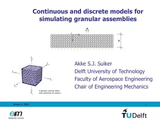
Continuous and discrete models for simulating granular assemblies. Akke S.J. Suiker Delft University of Technology Faculty of Aerospace Engineering Chair of Engineering Mechanics. Configuration of Lattice. Graphical representation of 9-cell square lattice model.

E N D
Continuous and discrete models for simulating granular assemblies Akke S.J. Suiker Delft University of Technology Faculty of Aerospace Engineering Chair of Engineering Mechanics
Configuration of Lattice Graphical representation of 9-cell square lattice model Suiker, Metrikine, de Borst, Int. J. Sol. Struct,38, 1563-1583, 2001 Suiker & de Borst, Phil. Trans. Roy. Soc. A., 363, 2543-2580, 2005
Long-wave approximation of EOM(I.A. Kunin, 1983) Replace discrete kinematic d.o.f.’s by continuous field variables: Replace discrete d.o.f.’s of neighbouring cells by second-order Taylor approximations of continuous field variables:
Equations of motion for Cosserat continuum (Cosserat E., Cosserat F., 1909; Günther, W., 1958; Schaefer, H., 1962; Mindlin, R.D., 1964; Eringen, A.C., 1968; Mühlhaus, H.-B., 1989; de Borst, R., 1991) • The Cosserat continuum model is useful for studying: • Localised failure problems, where rotation of grains is important • High-frequency wave propagation, with deformation patterns of short wavelengths
Mapping long-wave approximation on Cosserat model Relation between continuum material parameters and lattice parameters: Constraints that have to be satisfied to match the anisotropic lattice model with the isotropic Cosserat continuum model:
Configuration reduced lattice Graphical representation of reduced 9-cell square lattice model
Dispersion relations for plane harmonic waves Plane harmonic waves: Lattice Continuum Substitution into equations of motion yields: Dispersion relations:
Direction of propagation (kx,kz) = (0,k) Dispersion curves for 9-cell square lattice and Cosserat continuum
Second-gradient micro-polar model(microstructural approach) • Constitutive coefficients are of the form (using ) Suiker, de Borst, Chang, Acta Mech.,149, 161-180, 2001 Suiker, de Borst, Chang, Acta Mech.,149, 181-200, 2001 Suiker & de Borst, Phil. Trans. Roy. Soc. A., 363, 2543-2580, 2005
Reduced forms of the second-gradient micro-polar model • Linear elastic model, C(1) to C(6) = 0,: • Second-gradient model, C(3) to C(6) = 0, (Chang & Gao, 1995): • Cosserat model, C(1), C(2) and C(4) = 0, (Chang & Ma, 1992):
Dispersion curves for various models Dispersion curves for compression wave, shear wave and micro-rotational wave
Boundary value problem • Layer of thickness H, consisting of equi-sized particles of diameter d • - forced vibration under moving load Suiker, Metrikine, de Borst, J. Sound Vibr.,240, 1-18, 2001 Suiker, Metrikine, de Borst, J. Sound Vibr.,240, 19-39, 2001
Cells of square lattice Inner cell Boundary cell
Response of layer to a moving load 4 boundary conditions (in Fourier domain): - boundary cells at top of layer subjected to moving load in z-direction and free of loading in x-direction - displacements at bottom of layer are zero (in x- and z-directions) Substituting harmonic displacements into these 4 boundary conditions gives: Solve above system, and transform solution to time domain by Inverse Fourier Transform (numerical).
Displacement profile (H=300mm) (uz taken at 0.2H below layer surface) Case 1 Case 2 Velocity dependence Case 3 Harmonic load
Model Configuration Cuboidal volume of randomly packed, equi-sized, cohesionless spheres (initial porosity is 0.382). Suiker & Fleck, J. Appl. Mech.,71, 350-358, 2004
Stress-strain Response at various Contact Friction Stress-strain response for various contact friction angles
Effect of Contact Friction on Sample Strength Macroscopic friction angle versus contact friction angle
Effect of Particle Redistribution • Three different kinematic conditions: • Particle sliding and particle rotation are allowed • Particle sliding is allowed, particle rotation is prevented • Particle sliding is allowed in correspondence with an affine deformationfield, particle rotation is prevented.
Stress-strain Responses left: Volumetric strain versus hydrostatic stress (volumetric deformation path ) right: Deviatoric strain versus deviatoric stress (deviatoric deformation path )
Collapse Contour in the Deviatoric Plane Left: Collapse contour for unconstrained and constrained particle rotation ( ) Right: Collapse contour for DEM model (unconstrained particle rotation) and various continuum models
Points of discussion • Higher-order continuum models approach discrete models accurately up to a certain wavelength of deformation • Higher-order continuum models may be unstable for small wavelengths; • remedy: inclusion of higher-order time derivatives • (and coupled time-space derivatives) • Deformations with wavelengths < few times the particle diameter can not be decribed accurately with continuum models • The number of constitutive coefficients increases drastically when continuum models are further kinematically enhanced (i.e., 4th-order, 6th-order etc.)