Download
1 / 17
180 likes | 301 Vues
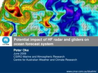
Potential impact of HF radar and gliders on ocean forecast system. Peter Oke June 2009 CSIRO Marine and Atmospheric Research Centre for Australian Weather and Climate Research. Talk Outline. NSW node of the Australian Integrated Marine Observing System Method

E N D
Potential impact of HF radar and gliders on ocean forecast system Peter Oke June 2009 CSIRO Marine and Atmospheric Research Centre for Australian Weather and Climate Research
Talk Outline • NSW node of the Australian Integrated Marine Observing System • Method • Assessment of Bluelink background and analysis error estimates • Estimation of likely analysis estimates with new observations • Summary & conclusions
HF radar x x X - mooring x x glider x approved wish-list Australian Integrated Marine Observing System: NSW node
1/10o 9/10o 2o The Bluelink System • Ocean Model • OFAM • MOM4p0d • Global model • 10 m vert res over top 200 m • Data Assimilation • BODAS • EnOI • 120 member ensemble • Localised covariances • Assimilates along-track ALTIM, coastal SLA, SST & in situ T and S
Method • To assimilate observations we must estimate: • the background error covariance (Pb) … errors in the model • the observation operator (H) … where & what the obs are • the observation error covariance (R) … errors in the obs • Given this information we can estimate: • the analysis error covariance (Pa) … errors in the analysis Pa= [I – PbHT(HPbHT + R)-1H] Pb • Bluelink uses an static ensemble, A = [a1a2 … an], to approximate Pb = AAT / (n-1). • The background ensemble A, with covariance Pb, can be efficiently transformed into the analysis ensemble Aa, with covariance Pa, using a transformation from ensemble square root filter theory. • This is most efficiently done serially – one observation at a time.
Assumed observation errors, R … includes instrument + representation error.
Experiments • We consider cases with: • GOOS + new platform • just new platform • just GOOS • Where the GOOS is assumed to be altimeters + SST + Argo/XBT
Impact of sampling error – varying obs distribution • Data distribution impacts the results – so we perform each calculation using the distribution of atSLA, SST and T/S from the GOOS for each week of 2006.
Evaluation of estimates: SLA • Estimated / Theoretical errors are based on the assumed and estimated BGF and analysis errors • Actual (BRAN) errors are computed from differences with observations over a 3-year reanalysis • Obs assimilated every 7-days include: • AMSRE SST • atSLA • Argo T/S • XBT
Assumed BGF errors and estimates analysis errors for all variables
Estimates % improvements for different HF radar arrays HF radar + GOOS % error reduction relative to GOOS with only ALTIM+SST+Argo HF radars are assumed to measure daily-mean surface velocity every day with no data gaps.
Actual glider path … not exactly the same as the assumed E-W tracks. Estimates % improvements for different glider sections (or CTD or mooring lines) Gliders + GOOS % error reduction relative to GOOS with only ALTIM+SST+Argo Gliders are assumed to “fly” along a fixed latitude within 200 km of the coast with a repeat cycles of 2-weeks.
Comparison of different options: showing analysis errors averaged over local regions
Conclusions • HF radar obs may reduce U/V errors by as much as 80%; and T/S and sea-level errors by ~60% near the observed regions. • T and S obs near the shelf are likely to provide a more modest benefit … because they are somewhat redundant. • assumed glider tracks are clearly unrealistic – and are more akin to repeat ship-borne CTD sections. • As a result of this study Bluelink will likely develop the capability to assimilate HF radar data (initially in research mode) once data is available – but will likely retain glider observations for validation. Sakov, P., and P. R. Oke 2008: Objective array design: Application to the tropical Indian Ocean. Journal of Atmospheric and Oceanic Technology,25, 794-807. Oke, P. R., P. Sakov and E. Schulz, 2009: A comparison of shelf observation platforms for assimilation into an eddy-resolving ocean model. Dynamics of Atmospheres and Oceans, in press.
Evaluation of estimates: SST • Estimated / Theoretical errors are based on the assumed and estimated BGF and analysis errors • Actual (BRAN) errors are computed from differences with observations over a 3-year reanalysis • Obs assimilated every 7-days include: • AMSRE SST • atSLA • Argo T/S • XBT