Download
1 / 12
120 likes | 326 Vues
Learn about Discrete Fourier Transform (DFT) and its applications, such as computing Continuous Fourier Transform (CFT) and Fourier Series. Compare DFT with CFT, understand windowing, sampling, and periodic sample generation. Discover how DFT can be used in computing complex Fourier series. Gain insights into spectral analysis using DFT and MATLAB.

E N D
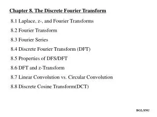
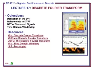
Chapter 2 Discrete Fourier Transform (DFT) Topics: • Discrete Fourier Transform. • Using the DFT to Compute the Continuous Fourier Transform. • Comparing DFT and CFT • Using the DFT to Compute the Fourier Series Huseyin Bilgekul Eeng360 Communication Systems I Department of Electrical and Electronic Engineering Eastern Mediterranean University
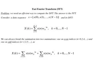
Where n = 0, 1, 2, …., N-1 where k = 0, 1, 2, …., N-1. Discrete Fourier Transform (DFT) • Definition: The Discrete Fourier Transform (DFT)is defined by: The Inverse Discrete Fourier Transform (IDFT) is defined by: The Fast Fourier Transform (FFT) is a fast algorithm for evaluating the DFT.
Using the DFT to Compute the Continuous Fourier Transform • Suppose the CFT of a waveform w(t) is to be evaluated using DFT. • The time waveform is first windowed (truncated) over the interval (0, T) so that only a finite number of samples, N, are needed. The windowed waveform ww(t) is • The Fourier transform of the windowed waveform is • Now we approximate the CFT by using a finite series to represent the integral, ∆t = T/N , t = k∆t, f = n/T, dt = ∆t
f = n/T and ∆t = T/N Computing CFT Using DFT • We obtain the relation between the CFT and DFT; that is, • The sample values used in the DFT computation are x(k) = w(k∆t), • If the spectrum is desired for negative frequencies – the computer returns X(n) for the positive n values of 0,1, …, N-1 – It must be modified to give spectral values over the entire fundamental range of -fs/2 < f <fs/2. For positive frequencies we use For Negative Frequencies
Comparisonof DFT and the Continuous Fourier Transform (CFT) Relationship between the DFT and the CFT involves three concepts: • Windowing, • Sampling, • Periodic sample generation
Comparisonof DFT and the Continuous Fourier Transform (CFT) Relationship between the DFT and the CFT involves three concepts: • Windowing, • Sampling, • Periodic sample generation
The Discrete Fourier Transform (DFT) may also be used to compute the complex Fourier series. • Fourier series coefficients are related to DFT by, Using the DFT to Compute the Fourier Series • Block diagram depicts the sequence of operations involved in approximating the FT with the DTFs.
Ex. 2.17 Use DFT to compute the spectrum of a Sinusoid Spectrum of a sinusoid obtained by using the MATLAB DFT.
Using the DFT to Compute the Fourier Series The DTFT and length-N DTFS of a 32-point cosine. The dashed line denotes the CFT. While the stems represent N|X[k]|. (a) N = 32 (b) N = 60 (c) N = 120.
Using the DFT to Compute the Fourier Series The DTFS approximation to the FT of x(t) = cos(2(0.4)t) + cos(2(0.45)t). The stems denote |Y[k]|, while the solid lines denote CFT. (a) M = 40. (b) M = 2000. (c) Behavior in the vicinity of the sinusoidal frequencies for M = 2000. (d) Behavior in the vicinity of the sinusoidal frequencies for M = 2010