Understanding Short Time Fourier Transform (STFT) Limitations & Applications
390 likes | 696 Vues
Explore the limitations of Fourier Transform and the advantages of STFT for analyzing non-stationary signals. Learn how STFT provides simultaneous time and frequency information, with steps and examples, emphasizing window selection and Heisenberg Principle.

Understanding Short Time Fourier Transform (STFT) Limitations & Applications
E N D
Presentation Transcript
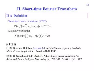
Short Time Fourier Transform (STFT) CS474/674 – Prof. Bebis (chapters 1 and 2 from Wavelet Tutorial posted on the web)
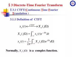
Fourier Transform (inverse DFT) where: (forward DFT) Fourier Transform reveals which frequency components are present in a given function.
Examples (cont’d) F1(u) F2(u) F3(u)
Limitations of Fourier Transform Poor localization in freq domain! Great localization in freq domain! 1. Cannot not provide simultaneous time and frequency localization.
Limitations of Fourier Transform (cont’d) Non-stationary signal (varying frequency) Stationary signal (non-varying frequency) 2. Not very useful for analyzing time-variant, non-stationary signals.
Limitations of Fourier Transform (cont’d) Three frequency components, present at all times! Three frequency components, NOT present at all times! F5(u) F4(u) Perfect knowledge of what frequencies exist, but no information about where these frequencies arelocated in time!
Limitations of Fourier Transform (cont’d) 3. Not efficient for representing non-smooth functions.
Representing discontinuities or sharp corners (cont’d) Original Reconstructed 1
Representing discontinuities or sharp corners (cont’d) Original Reconstructed 7
Representing discontinuities or sharp corners (cont’d) Original Reconstructed 23
Representing discontinuities or sharp corners (cont’d) Original Reconstructed 39
Representing discontinuities or sharp corners (cont’d) Original Reconstructed 128 coefficients 63
Representing discontinuities or sharp corners (cont’d) Original Reconstructed 95
Representing discontinuities or sharp corners (cont’d) Original Reconstructed 127 A large number of Fourier components is needed to represent discontinuities.
Short Time Fourier Transform (STFT) • Segment signal into narrow time intervals (i.e., narrow enough to be considered stationary) and take the FT of each segment. • Each FT provides the spectral information of a separate time-slice of the signal, providing simultaneoustime and frequency information.
STFT - Steps (1) Choose a window of finite length (2) Place the window on top of the signal at t=0 (3) Truncate the signal using this window (4) Compute the FT of the truncated signal, save results. (5) Incrementally slide the window to the right (6) Go to step 3, until window reaches the end of the signal
STFT - Definition frequency parameter time parameter 2D function windowing function centered at t=t’
Example f(t) [0 – 300] ms 75 Hz sinusoid [300 – 600] ms 50 Hz sinusoid [600 – 800] ms 25 Hz sinusoid [800 – 1000] ms 10 Hz sinusoid
Example f(t) [0 – 300] ms 75 Hz [300 – 600] ms 50 Hz [600 – 800] ms 25 Hz [800 – 1000] ms 10 Hz W(t) scaled: t/20
Choosing Window W(t) • What shape should it have? • Rectangular, Gaussian, Elliptic … • How wide should it be? • Should be narrow enough to ensure that the portion of the signal falling within the window is stationary. • Very narrow windows, however, do not offer good localization in the frequency domain.
STFT Window Size W(t) infinitely long: STFT turns into FT, providing excellentfrequency localization, but no time localization. W(t) infinitely short: results in the time signal (with a phase factor), providing excellenttime localization but no frequency localization.
STFT Window Size (cont’d) • Wide window good frequency resolution, poor time resolution. • Narrow window good time resolution, poor frequency resolution.
Example different size windows [0 – 300] ms 75 Hz [300 – 600] ms 50 Hz [600 – 800] ms 25 Hz [800 – 1000] ms 10 Hz
Example (cont’d) scaled: t/20
Example (cont’d) scaled: t/20
Heisenberg (or Uncertainty) Principle Time resolution:How well two spikes in time can be separated from each other in the frequency domain. Frequency resolution:How well two spectral components can be separated from each other in the time domain
Heisenberg (or Uncertainty) Principle • We cannot know the exact time-frequency representation of a signal. • We can only know what interval of frequencies are present in which time intervals.