Object Tracking
Babol university of technology. ECE Dep. Object Tracking. Machine Vision. Prof: M. Ezoji. Presentation: Alireza Asvadi. Winter 2012. What is tracking?. Estimating the trajectory of an object over time by locating its position in every frame.

Object Tracking
E N D
Presentation Transcript
Babol university of technology ECE Dep. Object Tracking Machine Vision Prof: M. Ezoji Presentation: AlirezaAsvadi Winter 2012
What is tracking? Estimating the trajectory of an object over time by locating its position in every frame. “Tracking by detection” Vs “Tracking with dynamics” Tracking by Detection: we have a strong model of the object, we detect the object independently in each frame and can record its position over time. Tracking with dynamics: we use object position estimated by measurement but also incorporate the position predicted by dynamics.
Tracking by detection: Time t Time t+1 Time t+n 1. detect the object independently in each frame 2. Link up the instances and we have a track Ref: Master Thesis, AlirezaAsvadi, "Object Tracking from Video Sequence (using color and texture information and RBF Networks)"
Methods for detection of object : Point detectors Template and density Based appearance models Background Modeling Background Subtraction Shape models Other Methods: Supervised Classifiers Contour evaluation …. Ref: Master Thesis, AlirezaAsvadi, "Object Tracking from Video Sequence (using color and texture information and RBF Networks)"
Start Take new image Select Good Features If lost features Yes Replace features Track Features No If images remaining Yes Replace features Store Image No Stop Point detectors: Point detectors are used to find interest points in images which have an expressive texture in their respective localities. The object is represented by points. commonly used interest point detectors include Moravec, Harris and SIFT detector. KLT control graph: Ref: Ankit Gupta (1999183) Vikas Nair (1999219) Supervisor Prof M. Balakrishnan Electrical Engineering Department IIT Delhi
Ref: M. Sonka,V. Hlavac, R.Boyle, “Image Processing, Analysis, and Machine Vision,” 3rd Edition, 2008. Ref: A. Yilmaz, O. Javed, and M. Shah, “Object tracking: A survey,” ACM Computing Surveys, Vol. 38, No. 4, pp. 1–45, December 2006.
I(x,y) O(x,y) Correlation x,y x,y Template Image Input Image Output Image Template Matching: Template matching is a brute force method of searching the image for a region similar to the object template. The position of the template in the current image is computed by a similarity measure, for example: NCC=normalized cross-correlation SSD=Sum of square differences SAD=Sum of absolute differences Ref: Ankit Gupta (1999183) Vikas Nair (1999219) Supervisor Prof M. Balakrishnan Electrical Engineering Department IIT Delhi
x is the template gray level image x is the average grey level in the template y is the source image section y is the average grey level in the source image N is the number of pixels in the section image (N= template image size = columns * rows) The value cor is between –1 and +1, with larger values representing a stronger relationship between the two images. Template Matching: NCC: In Matlab: C = normxcorr2(template, A) Affine Transformations could be use to Confirm a Match. Ref: M. Sonka,V. Hlavac, R.Boyle, “Image Processing, Analysis, and Machine Vision,” 3rd Edition, 2008.
Frame NCC Template SSD=sum((TEMP(:)-IMGBLK(:)).^2) SAD=sum(abs(TEMP(:)- IMGBLK(:)))
Shape Matching: Shape matching can be performed similar to tracking based on template matching. shape models are usually in the form of edge maps. Ref: A. Yilmaz, O. Javed, and M. Shah, “Object tracking: A survey,” ACM Computing Surveys, Vol. 38, No. 4, pp. 1–45, December 2006.
Background Subtraction: Background subtraction is often a good enough detector in applications where the background is known and all trackable objects look different from the background. The most important limitation of background subtraction is the requirement of stationary cameras. Ref: M. Sonka,V. Hlavac, R.Boyle, “Image Processing, Analysis, and Machine Vision,” 3rd Edition, 2008.
Supervised Classifiers: Object detection can be performed by learning different object views automatically from a set of examples by means of a supervised learning mechanism. During testing, the classifier gives a score to the test data indicating the degree of membership of the test data to the positive class. Maximum classification score over image regions estimate the position of the object. Ref: A. Yilmaz, O. Javed, and M. Shah, “Object tracking: A survey,” ACM Computing Surveys, Vol. 38, No. 4, pp. 1–45, December 2006.
See Details in Mean Shift Slides
Mean Shift Widely used, various enhancements (e.g. Robert Collins):
Problems with Tracking by detection Methods: Occlusions: Time Similar Objects:
Problems with Tracking by detection Methods: Or if the detector fails to detect object NCC map in First Frame (A template matching Example)
Tracking with dynamics: Observation (Detected object) + Dynamics Key idea: Given a model of expected motion, predict where objects will occur in next frame. • Prediction vs. correction • If the observation model is too strong, tracking is reduced to repeated detection • If the dynamics model is too strong, will end up ignoring the data
Filtering Problem: Estimate of c based on Prediction a and measurement b In kalman Filter they are correspond with:
Kalman filter assumptions: The Kalman filter model assumes that the state of a system at a time t evolved from the prior state at time t-1 according to: Measurements of the system can be performed, according to the model: To have similar notation R. Faragher , “Understanding the Basis of the Kalman Filter Via a Simple and Intuitive Derivation,” IEEE Signal Processing Magazine, September 2012.
The Kalman filter: state vector: (position & velocity) Control information: (force) The relationship between the force During the time period Δt and position and velocity: In matrix form: R. Faragher , “Understanding the Basis of the Kalman Filter Via a Simple and Intuitive Derivation,” IEEE Signal Processing Magazine, September 2012.
The Kalman filter: The information from the predictions and measurements are combined to provide the best possible estimate of the location of the train. THE PRODUCT OF TWO GAUSSIAN FUNCTIONS IS ANOTHER GAUSSIAN FUNCTION R. Faragher , “Understanding the Basis of the Kalman Filter Via a Simple and Intuitive Derivation,” IEEE Signal Processing Magazine, September 2012.
The Kalman filter: R. Faragher , “Understanding the Basis of the Kalman Filter Via a Simple and Intuitive Derivation,” IEEE Signal Processing Magazine, September 2012.
The Kalman filter: R. Faragher , “Understanding the Basis of the Kalman Filter Via a Simple and Intuitive Derivation,” IEEE Signal Processing Magazine, September 2012.
Read details in References process noise covariance Estimate (a posteriori) Best Prediction prior to Zk (a priori) Optimal Weighting (Kalman Gain) Residual G. Welch, G. Bishop , “An Introduction to the Kalman Filter,” ,1995.
The Kalman filter: Small measurement error: The observation model is too strong, tracking is reduced to repeated detection Small prediction error: the dynamics model is too strong, will end up ignoring the data
The Kalman filter: G. Welch, G. Bishop , “An Introduction to the Kalman Filter,” ,1995.
Problems: Yet it is not good enough Kalman filter Estimate Is combination of Prediction and Measurement. Till now we considered the entire measurements But what if we omit uninformative observations or highly unlikely measurements? It is Data Association. Result by applying The kalman filter
Data association: So far, we’ve assumed the entire measurement to be relevant to determining the state. In reality, there may be uninformative measurements or measurements that are not necessarily resulted from the target of interest or may belong to different tracked objects. Data association: task of determining which measurements go with which tracks. Simple strategy: only pay attention to the measurement that is “closest” to the prediction.
Tracking: Detection(observation)+ dynamics +Data association DA(Gating): Omit Measurements Outside the gate (say a circle with radius 50) Applying Data association (Gating) Notice Predicted Values By Kalman Filter (Green)
Summary: Tracking by detection detect the object independently in each frame tracking=Detection Detection Methods: Tracking with dynamics incorporate object dynamics to tracking Methods: tracking=Detection(observation)+dynamics Applying Data association Eliminate highly unlikely measurements tracking=Detection(observation)+ dynamics +Data association Point detectors Template matching density Based appearance models Shape models Background Subtraction … Filtering Methods Kalman filter … Tracking Matching Gating … Methods:
Reference: D. A. Forsyth, J. Ponce, “Computer Vision: A Modern Approach,” Prentice Hall,2nd Edition, 2012. M. Sonka,V. Hlavac, R.Boyle, “Image Processing, Analysis, and Machine Vision,” 3rd Edition, 2008. A. Yilmaz, O. Javed, and M. Shah, “Object tracking: A survey,” ACM Computing Surveys, Vol. 38, No. 4, pp. 1–45, December 2006. R. Faragher , “Understanding the Basis of the Kalman Filter Via a Simple and Intuitive Derivation,” IEEE Signal Processing Magazine, September 2012. G. Welch, G. Bishop , “An Introduction to the Kalman Filter,” ,1995.