Download
1 / 41
430 likes | 764 Vues
Formal Definition. A basic expression in the relational algebra consists of either one of the following: A relation in the database A constant relation Let E 1 and E 2 be relational-algebra expressions; the following are all relational-algebra expressions: E 1 E 2 E 1 - E 2

E N D
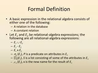
Formal Definition • A basic expression in the relational algebra consists of either one of the following: • A relation in the database • A constant relation • Let E1 and E2 be relational-algebra expressions; the following are all relational-algebra expressions: • E1 E2 • E1 - E2 • E1 x E2 • p (E1), P is a predicate on attributes in E1 • s(E1), S is a list consisting of some of the attributes in E1 • x(E1), x is the new name for the result of E1
Additional Operations We define additional operations that do not add any power to the relational algebra, but that simplify common queries. • Set intersection • Natural join • Division • Assignment
Set-Intersection Operation • Notation: r s • Defined as: • rs ={ t | trandts } • Assume: • r, s have the same arity • attributes of r and s are compatible • Note: rs = r - (r - s)
Set-Intersection Operation - Example A B A B • Relation r, s: • r s 1 2 1 2 3 r s A B 2
Natural-Join Operation • Notation: r s • Let r and s be relations on schemas R and S respectively.The result is a relation on schema R S which is obtained by considering each pair of tuples tr from r and ts from s. • If tr and ts have the same value on each of the attributes in RS, a tuple t is added to the result, where • t has the same value as tr on r • t has the same value as ts on s • Example: R = (A, B, C, D) S = (E, B, D) • Result schema = (A, B, C, D, E) • rs is defined as: r.A, r.B, r.C, r.D, s.E (r.B = s.B r.D = s.D (r x s))
r s Natural Join Operation – Example • Relations r, s: B D E A B C D 1 3 1 2 3 a a a b b 1 2 4 1 2 a a b a b r s A B C D E 1 1 1 1 2 a a a a b
Division Operation r s • Suited to queries that include the phrase “for all”. • Let r and s be relations on schemas R and S respectively where • R = (A1, …, Am, B1, …, Bn) • S = (B1, …, Bn) The result of r s is a relation on schema R – S = (A1, …, Am) r s = { t | t R-S(r) u s ( tu r ) }
Division Operation – Example A B Relations r, s: B 1 2 3 1 1 1 3 4 6 1 2 1 2 s r s: A r
Another Division Example Relations r, s: A B C D E D E a a a a a a a a a a b a b a b b 1 1 1 1 3 1 1 1 a b 1 1 s r A B C r s: a a
Division Operation (Cont.) • Property • Let q – r s • Then q is the largest relation satisfying q x s r • Definition in terms of the basic algebra operationLet r(R) and s(S) be relations, and let S R r s = R-S (r) –R-S ( (R-S(r) x s) – R-S,S(r)) To see why • R-S,S(r) simply reorders attributes of r • R-S(R-S(r) x s) – R-S,S(r)) gives those tuples t in R-S(r) such that for some tuple u s, tu r.
Assignment Operation • The assignment operation () provides a convenient way to express complex queries, write query as a sequential program consisting of a series of assignments followed by an expression whose value is displayed as a result of the query. • Assignment must always be made to a temporary relation variable. • Example: Write r s as temp1 R-S (r)temp2 R-S ((temp1 x s) – R-S,S(r))result = temp1 – temp2 • The result to the right of the is assigned to the relation variable on the left of the . • May use variable in subsequent expressions.
Example Queries • Find all customers who have an account from at least the “Downtown” and the Uptown” branches. • Query 1 CN(BN=“Downtown”(depositoraccount)) CN(BN=“Uptown”(depositoraccount)) where CN denotes customer-name and BN denotes branch-name. • Query 2 customer-name, branch-name(depositoraccount) temp(branch-name) ({(“Downtown”), (“Uptown”)})
Example Queries • Find all customers who have an account at all branches located in Brooklyn city.customer-name, branch-name(depositoraccount) branch-name(branch-city = “Brooklyn”(branch))
Extended Relational-Algebra-Operations • Generalized Projection • Outer Join • Aggregate Functions
Generalized Projection • Extends the projection operation by allowing arithmetic functions to be used in the projection list.F1, F2, …, Fn(E) • E is any relational-algebra expression • Each of F1, F2, …, Fn are are arithmetic expressions involving constants and attributes in the schema of E. • Given relation credit-info(customer-name, limit, credit-balance), find how much more each person can spend: customer-name, limit – credit-balance (credit-info)
Aggregate Functions and Operations • Aggregation function takes a collection of values and returns a single value as a result. avg: average valuemin: minimum valuemax: maximum valuesum: sum of valuescount: number of values • Aggregate operation in relational algebra G1, G2, …, GngF1( A1), F2( A2),…, Fn( An) (E) • E is any relational-algebra expression • G1, G2 …, Gn is a list of attributes on which to group (can be empty) • Each Fiis an aggregate function • Each Aiis an attribute name
Aggregate Operation – Example A B C • Relation r: 7 7 3 10 sum-C gsum(c)(r) 27
Aggregate Operation – Example • Relation account grouped by branch-name: branch-name account-number balance Perryridge Perryridge Brighton Brighton Redwood A-102 A-201 A-217 A-215 A-222 400 900 750 750 700 branch-nameg sum(balance) (account) branch-name balance Perryridge Brighton Redwood 1300 1500 700
Aggregate Functions (Cont.) • Result of aggregation does not have a name • Can use rename operation to give it a name • For convenience, we permit renaming as part of aggregate operation branch-nameg sum(balance) as sum-balance (account)
Outer Join • An extension of the join operation that avoids loss of information. • Computes the join and then adds tuples form one relation that does not match tuples in the other relation to the result of the join. • Uses null values: • null signifies that the value is unknown or does not exist • All comparisons involving null are (roughly speaking) false by definition. • Will study precise meaning of comparisons with nulls later
Outer Join – Example • Relation loan branch-name loan-number amount Downtown Redwood Perryridge L-170 L-230 L-260 3000 4000 1700 • Relation borrower customer-name loan-number Jones Smith Hayes L-170 L-230 L-155
loan-number branch-name amount customer-name L-170 L-230 Downtown Redwood 3000 4000 Jones Smith Outer Join – Example • Inner Joinloan Borrower • Left Outer Join loan borrower loan-number branch-name amount customer-name L-170 L-230 L-260 Downtown Redwood Perryridge 3000 4000 1700 Jones Smith null
Outer Join – Example • Right Outer Join loanborrower loan-number branch-name amount customer-name L-170 L-230 L-155 Downtown Redwood null 3000 4000 null Jones Smith Hayes • Full Outer Join loan borrower loan-number branch-name amount customer-name L-170 L-230 L-260 L-155 Downtown Redwood Perryridge null 3000 4000 1700 null Jones Smith null Hayes
Null Values • It is possible for tuples to have a null value, denoted by null, for some of their attributes • null signifies an unknown value or that a value does not exist. • The result of any arithmetic expression involving null is null. • Aggregate functions simply ignore null values • Is an arbitrary decision. Could have returned null as result instead. • We follow the semantics of SQL in its handling of null values • For duplicate elimination and grouping, null is treated like any other value, and two nulls are assumed to be the same • Alternative: assume each null is different from each other • Both are arbitrary decisions, so we simply follow SQL
Null Values • Comparisons with null values return the special truth value unknown • If false was used instead of unknown, then not (A < 5) would not be equivalent to A >= 5 • Three-valued logic using the truth value unknown: • OR: (unknownortrue) = true, (unknownorfalse) = unknown (unknown or unknown) = unknown • AND: (true and unknown) = unknown, (false and unknown) = false, (unknown and unknown) = unknown • NOT: (not unknown) = unknown • In SQL “P is unknown” evaluates to true if predicate P evaluates to unknown • Result of select predicate is treated as false if it evaluates to unknown
Modification of the Database • The content of the database may be modified using the following operations: • Deletion • Insertion • Updating • All these operations are expressed using the assignment operator.
Deletion • A delete request is expressed similarly to a query, except instead of displaying tuples to the user, the selected tuples are removed from the database. • Can delete only whole tuples; cannot delete values on only particular attributes • A deletion is expressed in relational algebra by: r r – E where r is a relation and E is a relational algebra query.
Deletion Examples • Delete all account records in the Perryridge branch. account account – branch-name = “Perryridge” (account) • Delete all loan records with amount in the range of 0 to 50 loan loan – amount 0and amount 50 (loan) • Delete all accounts at branches located in Needham. r1 branch-city = “Needham”(account branch) r2 branch-name, account-number, balance (r1) r3 customer-name, account-number(r2 depositor) account account – r2 depositor depositor – r3
Insertion • To insert data into a relation, we either: • specify a tuple to be inserted • write a query whose result is a set of tuples to be inserted • in relational algebra, an insertion is expressed by: r r E where r is a relation and E is a relational algebra expression. • The insertion of a single tuple is expressed by letting E be a constant relation containing one tuple.
Insertion Examples • Insert information in the database specifying that Smith has $1200 in account A-973 at the Perryridge branch. account account {(“Perryridge”, A-973, 1200)} depositor depositor {(“Smith”, A-973)} • Provide as a gift for all loan customers in the Perryridge branch, a $200 savings account. Let the loan number serve as the account number for the new savings account. r1 (branch-name = “Perryridge” (borrower loan)) account account branch-name, account-number,200 (r1) depositor depositor customer-name, loan-number,(r1)
Updating • A mechanism to change a value in a tuple without charging all values in the tuple • Use the generalized projection operator to do this task r F1, F2, …, FI, (r) • Each F, is either the ith attribute of r, if the ith attribute is not updated, or, if the attribute is to be updated • Fi is an expression, involving only constants and the attributes of r, which gives the new value for the attribute
Update Examples • Make interest payments by increasing all balances by 5 percent. account AN, BN, BAL * 1.05(account) where AN, BNand BALstand for account-number, branch-name and balance, respectively. • Pay all accounts with balances over $10,0006 percent interest and pay all others 5 percent account AN, BN, BAL * 1.06( BAL 10000 (account)) AN, BN, BAL * 1.05 (BAL 10000 (account))
Views • In some cases, it is not desirable for all users to see the entire logical model (i.e., all the actual relations stored in the database.) • Consider a person who needs to know a customer’s loan number but has no need to see the loan amount. This person should see a relation described, in the relational algebra, by customer-name, loan-number (borrower loan) • Any relation that is not of the conceptual model but is made visible to a user as a “virtual relation” is called a view.
View Definition • A view is defined using the create view statement which has the form create view v as <query expression where <query expression> is any legal relational algebra query expression. The view name is represented by v. • Once a view is defined, the view name can be used to refer to the virtual relation that the view generates. • View definition is not the same as creating a new relation by evaluating the query expression Rather, a view definition causes the saving of an expression to be substituted into queries using the view.
View Examples • Consider the view (named all-customer) consisting of branches and their customers. create view all-customer as branch-name, customer-name (depositor account) branch-name, customer-name(borrowerloan) • We can find all customers of the Perryridge branch by writing: branch-name (branch-name = “Perryridge” (all-customer))
Tuple Relational Calculus • A nonprocedural query language, where each query is of the form {t | P (t) } • It is the set of all tuples t such that predicate P is true for t • t is a tuple variable, t[A] denotes the value of tuple t on attribute A • t r denotes that tuple t is in relation r • P is a formula similar to that of the predicate calculus
Predicate Calculus Formula 1. Set of attributes and constants 2. Set of comparison operators: (e.g., , , , , , ) 3. Set of connectives: and (), or (v)‚ not () 4. Implication (): x y, if x if true, then y is true x y x v y 5. Set of quantifiers: • t r (Q(t)) ”there exists” a tuple in t in relation r such that predicate Q(t) is true • t r (Q(t)) Q is true “for all” tuples t in relation r
Banking Example • branch (branch-name, branch-city, assets) • customer (customer-name, customer-street, customer-city) • account (account-number, branch-name, balance) • loan (loan-number, branch-name, amount) • depositor (customer-name, account-number) • borrower (customer-name, loan-number)
Example Queries • Find the loan-number, branch-name, and amount for loans of over $1200 {t | t loan t [amount] 1200} • Find the loan number for each loan of an amount greater than $1200 {t | s loan (t[loan-number] = s[loan-number] s [amount] 1200} Notice that a relation on schema [customer-name] is implicitly defined by the query
Example Queries • Find the names of all customers having a loan, an account, or both at the bank {t | s borrower(t[customer-name] = s[customer-name]) u depositor(t[customer-name] = u[customer-name]) • Find the names of all customers who have a loan and an account at the bank {t | s borrower(t[customer-name] = s[customer-name]) u depositor(t[customer-name] = u[customer-name])
Example Queries • Find the names of all customers having a loan at the Perryridge branch {t | s borrower(t[customer-name] = s[customer-name] u loan(u[branch-name] = “Perryridge” u[loan-number] = s[loan-number]))} • Find the names of all customers who have a loan at the Perryridge branch, but no account at any branch of the bank {t | s borrower(t[customer-name] = s[customer-name] u loan(u[branch-name] = “Perryridge” u[loan-number] = s[loan-number])) not v depositor (v[customer-name] = t[customer-name]) }