Download
1 / 135
1.38k likes | 1.85k Vues
27-09-2012 Data mining. Sven Kouwenhoven Adam Swarek Chantal Choufoer. K-nearest neighbor & Naive Bayes. General Plan. Part 1 Discuss K-nearest neighbor & Naive Bayes 1 Method 2 Simple example 3 Real life example Part 2 Application of the method to the Charity Case

E N D
27-09-2012 Data mining Sven Kouwenhoven Adam Swarek Chantal Choufoer K-nearest neighbor & Naive Bayes
General Plan Part 1 Discuss K-nearest neighbor & Naive Bayes 1 Method 2 Simple example 3 Real life example Part 2 Application of the method to the Charity Case Information about the case Pre-analysis of the data 1 Data visualization 2 Data reduction Analysis 1 Recap of the method 2 How do we apply the method to the case 3 The result of the model 4 Choice of the variables 5 Conclusion and recommendations for the client Conclusion
K-NN K – nearest neighbors
General info • You can have either numerical or categorical outcome – we focus on categorical (classification as opposed to prediction) • Non-parametric - does not involve estimation of parameters in a function form • In practice – it doesnt give you a nice equation that you can apply readily, each time you have to go back to the whole dataset.
K-NN – basic idea • „K” stands for the number of nearest neighbours you want to have evaluated • „Majority vote” – You evaluate the „k” nearest neighbors and count which label occurs more frequently and you choose this label
Which one actually is the nearest neghbour? • The one that basically is the closest - most frequently euclidean distance used to measure it: • p – • X – • U - • A lot of other variations • E.g • Different weights • Other types of distance measures
How to choose K ? • No single way to do this • Not too high • Otherwise you will not capture the local structure of data, which is one of the biggest advantages of k-nn • Not too low • Otherwise you will capture the noise in the data . • So what to do ? • Play with different values of k and see what gives you the most satisfying result • Avoid the values of k and multiples of kthat equal the number of possible outcomes of the predicted variables
Probability of given outcome • It is also possible to calculate probability of the given outcome basing on k-nn method • You simple take k nearest neighbors and count how many of them are in particular class and then the probability of a new record to belong to the class is the count number divided by k
PROS vs CONS • PROS: + Conceptual simplicity + Lack of parrametric assumptions no time required to estimate parameters from training data + Captures local structure of dataset + Training Dataset can be extended easily as opposed to parametric models, where probably new parameters would have to be developed or at least model would need testing
CONS - No general model in the form of eqation is given – each time we want to test the new data, the whole dataset has to be analyzed (slow) – processing time in large data set can be unacceptable but: - reduce directions - find „almost nearest neighbor” – sacrifice part of the accuracy for processing speed - Curse of dimensionality – data needed increases exponentially with number of predictors. ( large dataset required to give meaningful prediction )
Examplary uses • Nearest Neigbor based content retrieval ( in general product reccomandation ) - Amazon - detailed ex. - Pandora 2. Biological uses - Gene expression - Protein- Protein interaction Source: http://saravananthirumuruganathan.wordpress.com/2010/05/17/a-detailed-introduction-to-k-nearest-neighbor-knn-algorithm/ http://bionicspirit.com/blog/2012/01/16/cosine-similarity-euclidean-distance.html
How does it work ? (simplified) • Every song is assessed on hundreds of variables on scale from 0-5 by musicians • Each song is assigned a vector consisting of results on each variable • The user of the Radio chooses the song he/she likes ( the song has to be in Pandora’s database) • The program gives the suggested next song that would appeal ( based on the k-nn classification) to the taste of the person • The user marks as either „like” or „dislike” - the system keeps the information and can give another suggestion ( now based on the average of two liked songs ) of a song • The process follows and the program can give a better suggestion everytime.
Introductionto the method • Naive Bayes • Classification method • Maximize overall classification accuracy • Identifying records belonging to a particular class of interest • ‘Assigning to the most probable class’ method • Cutoff probability method
Introduction to the method Naive Bayes • ‘Assigning to the most probable class’ method 1 Find all the other records just like it 2 Determine what classes they all belong to an which class is more prevalent 3 Assign that class to the new record
Introduction to the method Naive Bayes 1 Establish a cutoff probability for the class of interest above which we consider that a record belongs to that class 2 Find all the training records just like the new record 3 Determine the probability that those records belong to the class of interest 4 If that probability is above the cutoff probability, assign the new record to the class of interest
Introductionto the method • Naive Bayes • Class conditional probability • Bayes Theorem: Prob(A given B) • A represents the dependent event and B represents the prior event. • * Bayes’ Theorem finds the probability of an event occurring given the probability of another event that has already occurred
Introductionto the method P(Ci|x1,….,xp) ; The probability of the record belonging to class i given that its predictor values take on the values x1,….xp Pnb (c1|x1,….,x2) =
Introduction to the method Naive Bayes • Categorical predictors: The Bayesian classifier works only with categorical predictors If we use a set of numerical predictors, what will happen? • Naive rule: assign all records to the majority class
Introduction to the method Naive Bayes • Advantages • Good classification performance • Computationally efficient • Binary and multiclass problems • Disadvantages • Requires a very large number of records • When the goal is estimating probability instead of classification, then the method provides a very biased results
NaiveBayesclassifier casethe training set P(Play_tennis) = 9/14 P(Don’t_play_tennis) = 5/14
Case: Should we play tennis today? Today the outlook is sunny, the temperature is cool, the humidity is high, and the wind is strong. X = (Outlook=Sunny, Temperature=Cool, Humidity=High, Wind=Strong)
Resultsforplaying P(Outlook=Sunny | Play=Yes) =X1 = 2/9 P(Temperature=Cool | Play=Yes) = X2 = 3/9 P(Humidity=High | Play=Yes) = X3 = 3/9 P(Wind=Strong | Play=Yes) = X4 = 3/9 P(Play=Yes) = P(CY) = 9/14
Numerator of naive Bayes equation P(X1|CY)* P(X2|CY)* P(X3|CY)* P(X4|CY)*P(CY)= (2/9) * (3/9) * (3/9) * (3/9) * (9/14) = 0.0053 0.0053 represents P(X1,X2,X3,X4|CY)*P(CY), which is the top part of the naive Bayes classifierformula
Resultsfornotplaying P(Outlook=Sunny | Play=No) = X1 = 3/5 P(Temperature=Cool | Play=No) = X2 = 1/5 P(Humidity=High | Play=No) = X3 = 4/5 P(Wind=Strong | Play=No) = X4 = 3/5 P(Play=No) = P(CN) = 5/14 (3/5) * (1/5) * (4/5) * (3/5) * (5/14) = 0.0206
Summary of the resultssofar For playing tennis, P(X1,X2,X3,X4|CY)P(CY) = 0.0053 For notplaying tennis P(X1,X2,X3,X4|CN)P(CN) = 0.0206
Denominator of naive Bayes equation Evidence = P(X1,X2,X3,X4|CY)*P(CY) + P(X1,X2,X3,X4|CN)*P(CN) = 0.0053 + 0.0206 = 0.0259
Answer: The probability of notplaying tennis is largerso we shouldnotplay tennis today.
Examplary uses • Text classifications • Spam filtering in E-mails • Text processors – errors correction • Detecting the language of the text • http://bionicspirit.com/blog/2012/02/09/howto-build-naive-bayes-classifier.html • Metereorology ( CALIPSO , PATMOS-x) • http://journals.ametsoc.org/doi/pdf/10.1175/JAMC-D-11-02.1 • Plagiarism detection
How does it work ? • Humans classify a huge amount of e-mails as spam or not spam, and then select equal training dataset of spam and non-spam emails. • For each word compute the frequency of occurance in spam and non-spam e-mails and attach probability of occurance of a word in spam as well as non-spam e-mail • Then apply the naive bayes probability of belonging to the class ( spam or not spam ) • Eihter the simple higher probability method or a cutoff threshold method to classify. • Additional – if you for example classify the e-mails in your e-mail client for spam and non spam, then you also create a personalized spam filter.
Part 2 • Application of the method to the charity case
General Introduction of the case • Dutch charity organization that wants to be able to classify it's supporters to donators and non-donators. • Goal of the charity organization - how will they meet the goal? Effective marketing : more direct marketing to highly potential customers
General Introduction of the case • Variable: TimeLr Time since last response TimeCl Time as client FrqRes Frequency of response MedTOR Median of time response AvgDon Average donation LstDon Last donation AnnDon Average annual donation DonInd Donation indicator in the considered mailing
General Introduction of the case The sample of the training data consist of 4057 customers The sample of the test data consist of 4080 customers
General Introduction of the case Assumptions Sending cost of the catalogue: € 0.50 Catalogue cost: € 2.50 Revenue of sending a catalogue to a donator: € 18,-
Application of the case • Evaluating performance Classificationmatrix Summarizes the correct and incorrect classifications that a classifier produced for a certain dataset • Sensitivity ability to detect the donators correctly - Specificity ability to rule out non-donators correctly Lift chart X-axis cumulative number of cases Y-axis cumulative number of true donators
Histogram forattribute TIMELR Y-axis: Number of peoplewhodonated X-axis: Time since last response in WEEKS
Histogram forattribute AVGDON Y-axis: Number of peoplewhodonated X-axis: Average amountthatpeopledonated