Initial Data Analysis
Initial Data Analysis. Beginning the Visualization of Data. Plotting Data. Often, the first thing one does with data is to plot frequency distributions.

Initial Data Analysis
E N D
Presentation Transcript
Initial Data Analysis Beginning the Visualization of Data
Plotting Data • Often, the first thing one does with data is to plot frequency distributions. • Usually this is done by first creating a table of the frequencies broken down by values of the relevant variable, then the frequencies in the table are plotted in a histogram.
Frequency Data • Example: Age as estimated by a questionnaire in an undergraduate statistics class. • Frequencies were calculated by simply counting the number of subjects having the specified value for the age variable.
Grouping data • Plotting is easy when the variable of interest has a relatively small number of values (like our age variable did). • However, the values of a variable are sometimes more continuous, resulting in uninformative frequency plots if done in the above manner. • In this case we’ll use a grouped frequency distribution
Graphic Depiction of Frequency • Histogram • Similar to a bar chart with the only difference being that histograms are representative of continuous data. • Age example
Histogram Construction Class Interval Frequency 20-under 30 6 30-under 40 18 40-under 50 11 50-under 60 11 60-under 70 3 70-under 80 1
Frequency Polygon Class Interval Frequency 20-under 30 6 30-under 40 18 40-under 50 11 50-under 60 11 60-under 70 3 70-under 80 1
How many ‘bins’? • Various rules of thumb that could suffice • At least around 10 • Use natural breaks in the number system (e.g. every 5 or 10) • √N • However, you should ‘play with it’ • Change the bins until you feel you are getting a good sense of what the data is doing • Example
Advantages/Disadvantages • With the grouped frequency distributions and histograms we can take large data sets and make them much more manageable and easier to understand. • Also, it’s a very good way to spot possible troublesome cases (outliers) • However, we also lose information about individual data points.
It is possible to obtain the graphical advantage of grouping and still keep all of the information if stem & leaf plots are used. These plots are created by splitting a data point into that part associated with the ‘group’ and that associated with the individual point. For example, the numbers 180, 180, 181, 182, 185, 186, 187, 187, 189 could be represented as: 18 001256779 Using a stem and leaf offers several advantages It retains individual data points Displays large amounts of data well (compared to a normal frequency distribution) Provides a ‘graphical’ display of the data Disadvantage Kind of ugly Stem and Leaf Plots
86 77 91 60 55 76 92 47 88 67 23 59 72 75 83 77 68 82 97 89 81 75 74 39 67 79 83 70 78 91 68 49 56 94 81 Stem and Leaf Plots Stem Leaf Raw Data 2 3 4 5 6 7 8 9 3 9 7 9 5 6 9 0 7 7 8 8 0 2 4 5 5 6 7 7 8 9 1 1 2 3 3 6 8 9 1 1 2 4 7
Stem and Leaf Plots • Stem & leaf plots are especially nice for comparing distributions.
Density • Density, the height of a curve for a probability distribution, reflects areas of values that we would expect to be more or less likely and give a good sense of the variability in the data • The are often superimposed1 on histograms, but in general give us a sense of the same sort of information • Violin plots are a more recent development which combine boxplots and probability density distributions • Area under the curve = 1
Box-plots • Box and whisker plots (Tukey) are graphical representations of Interquartile Range1 • Hinges mark the IQR • The median is marked within the box • Inner Fences typically mark a point that falls 1.5*(IQR) below or above the hinge • Adjacent values are the closest data point to the inner fences without going beyond • Whiskers connect the adjacent values to the nearest quartile • Any outliers designated in some fashion • So with a Box and Whisker plot we get a sense of variability, skewness and possible outlier detection
Putting it all together: Violin Plots • Best of both worlds • Here we can see easily the ‘middle’ is near about a 90, but there is a negative skew that tells us that perhaps some noticeably struggled relative to the rest of the class
Terminology Related to Distributions • Often, frequency histograms tend to have a roughly symmetrical bell-shape and contain the property referred to as Normal or Gaussian.
Distributions • However one should note that symmetrical does not mean normal • More on that later • Sometimes (most?) the shape is not symmetrical • Even when the sample comes from a normal distribution • The term positive skew refers to the situation where the long “tail” of the distribution is to the right on a horizontal display, negative skew is when the “tail” is to the left. • Can you think of variables that would naturally be skewed in the population?
Scatterplots • Scatterplots allow us to show the relationship between two variables • While typically applied to continuous data, their application to grouped data can allow one to see how individual scores while comparing groups as a whole
Scatterplots Boring Much more informative
Comparing groups • Using the scatterplot and a little ‘jitter’, we can retain individual score information, get a sense of the distribution and still see mean differences • This graph is referred to as a strip chart • Could also, instead of reference lines at the means, plot confidence intervals
Plotting Interval Estimates • One must be careful in plotting confidence intervals such that they clearly show what is meant to be conveyed • Group means? • The statistical test regarding them? • Effect size? • The plot on the left shows regular group CIs, group inferential CIs, a CI for the difference between the group means, and a CI for the Cohen’s d regarding that difference in means
More on graphical display of data • A graphical approach to data has the capacity to display your ideas more quickly and make them more readily received • While the capacity to make great looking graphs is now available to us, the point is not just about ‘pretty pictures’ • We need to make our ideas clear, and use graphics appropriately to aid in that task • In other words make them as simple as possible without neglecting important aspects of the data