Download
1 / 35
350 likes | 514 Vues
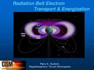
Recent Results from Theory and Modeling of Radiation Belt Electron Transport, Acceleration, and Loss. Anthony Chan, Bin Yu, Xin Tao, Richard Wolf Rice University Scot Elkington, Seth Claudepierre University of Colorado Jay Albert AFRL Michael Wiltberger NCAR.

E N D
Recent Results from Theory and Modeling of Radiation Belt Electron Transport, Acceleration, and Loss Anthony Chan, Bin Yu, Xin Tao, Richard Wolf Rice University Scot Elkington, Seth Claudepierre University of Colorado Jay Albert AFRL Michael Wiltberger NCAR REPW, Rarotonga, Cook Islands, August 7, 2007
OUTLINE 1. Radial Diffusion in High-Speed-Stream Storms 2. MHD-Particle Simulation of a HSS Storm 3. Multidimensional Diffusion Using SDEs
1. Radial Diffusion in High-Speed-Stream Storms [Bin Yu, PhD thesis, 2007] • Solve the standard radial diffusion equation, with loss term. • DLL from Brautigam and Albert [2000]. • Loss lifetime from Shprits et al [2004], and Meredith et al [2006]. • Dynamic outer boundary: Location = min(L_GEO, 0.9*L_last-closed) Outer boundary value from Li et al [2001] GEO model. Fixed inner boundary: L=2, value from AE8MIN • Initial condition from AE8MIN. • Magnetic field: Hilmer and Voigt [1995]. For comparison: Tsyganenko 2001, dipole
Some Details of the Radial Diffusion Model • M: 20 MeV/G ~ 6000MeV/G, 100 bins • L: 2~7, 100 bins • Time Steps: 4min. Total time: 6 days • Method: Crank-Nicholson implicit method Our approach: • Consider a model HSS storm in declining phase of the solar cycle • Compare with a series of HSS events, between 1995 and 1996, published by Hilmer et al [2000].
A Typical High-Speed-Stream Storm Solar wind parameters and indices for the January 1995 high-speed stream (HSS) storm:
Solar Wind Parameters for a Model High-Speed-Stream Storm Schematic illustration of a CIR [Pizzo, 1978]. Input parameters for our idealized declining phase magnetic storm: (a) solar wind density n (cm-3), (b) solar wind velocity V (km/s), (c) IMF Bz (nT), (d) solar wind ram pressure P (nPa), (e) Dst index, (f) Kp index, (g) midnight equatorward boundary of the aurora.
Electron Lifetime Model • Plasmapause location: Lpp = 5.6 – 0.46 Kp [Carpenter and Anderson, JGR, 1992] • Outside the plasmapause: Use a Kp-dependent lifetime of electron loss from Shprits et al, GRL, 2004. I.e., 0.5 day during storm main phase (Kp=6), 3 days under quiet conditions (Kp=2), and linearly dependent on Kp. GEO to GPS is mostly outside the plasmapause for HSS events. • Inside the plasmapause: * Estimate the recovery-phase electron lifetime based on CRRES measurements [Meredith et al., JGR, 2006]. * Assume typical VLF wave amplitudes of 10pT and 35pT and multiply the lifetime by (10/35)2 to get the main-phase lifetime.
PSD f(R,M,t) Results for the January 1995 Event • Compare simulation results with observations. • Middle simulation results exhibit similar shape with observations, but diffusion is too fast. • Lowering DLL by a factor of two gives better agreement. Six-hour averages of PSD from observations [Hilmer et al., 2000] for Julian Day 28-34, 1995; Simulation result using similar solar wind condition and Brautigam and Albertformula of DLL. Simulation result using DLL/2.
PSD f(R,M,t) Results for the July 1995 Event • Another high-speed-stream event : The July 1995 storm event • No growth of phase space density at R = 4.2 Re is observed • Average Kp during the recovery phase is about 3 • Again, better agreement with observations is obtained if we divide the Brautigam and Albert diffusion coefficient by 2. Observations DLL DLL/2
Reasonable agreement is obtained between measured and simulated rate-of-increase of PSD at GPS, using B&A DLL divided by 2(±0.5).
Radial Diffusion in High-Speed-Stream Storms: Summary • Enhancement of MeV electrons at R ≈ 4 during high-speed-stream storms is well reproduced by radial diffusion modeling. • Diffusion can transport electrons efficiently to lower L from a source region near L=6.6Re, consistent with the GPS data. • If we artificially divide the Brautigam and Albert [200] formula for DLL by a factor of 2, the simulation results reproduced the Hilmer et al. [2001] observations well.
OUTLINE 1. Radial Diffusion in High-Speed-Stream Storms 2. MHD-Particle Simulation of a HSS Storm 3. Multidimensional Diffusion Using SDEs
2. MHD-Particle Simulation of a HSS Storm: Overview A. MHD-Particle Simulation B. Phase-Space Density Evolution C. Radial Diffusion Coefficients Summary [Bin Yu, PhD thesis, 2007]
A. MHD-Particle Simulation • The LFM global MHD code is driven by solar-wind inputs for the Jan 1995 high-speed-stream (HSS) storm: • Equatorial particles are traced by solving relativistic guiding-center equations of Brizard and Chan[Phys. Plasmas, 1999].
MHD-Particle Simulation Results • Black lines: Constant-B contours. Dashed circles: 3, 5, 7,… RE Color: particle energy, M = 2100 MeV/G • Particle boundaries at 3.5 RE and 10 RE Reference for MHD-particle method: Elkington et al, JASTP, 2002.
MHD-Particle Simulation Results: Snapshots • From pre-storm to late recovery phase (top L to R, bottom L to R) • Magnetopause loss occurs early in Jan 29 (between panels 2 and 3)
B. Phase-Space Density Evolution Overview of Method: • Use Liouville’s theorem, regard GC particles as “markers”. • Initial PSD f is scaled from AE8 empirical model. • Step markers in time with GC equations of motion. • PSD f is conserved along each marker trajectory. • Recalculate PSD f on an equatorial grid using an area-weighting scheme [Nunn, J. Comp. Phys., 1993] …
Q1 Q2 A3 A4 PSD marker A2 A1 Q4 Q3 The phase-space density (PSD) weighting scheme The contribution of each marker to the total phase-space density is calculated on the grid using an area-weighting formula:
Advantages of this PSD-evolution algorithm: • Low noise level and efficient use of particles/markers. • The resulting PSD f is always non-negative. (Negative values can be a problem in PDE solvers.) • A variety of boundary conditions can be implemented. • E.g., markers at or outside GEO may be assigned the observed GEO phase-space density. • New markers can be added, if needed (but marker weights have to be carefully “re-normalized”) • A loss lifetime can be used to decrease PSD at each grid point, at each time step.
Phase-Space Density Results I • Observed (blue) and simulated (red) electron PSD. Solid line = GEO, dashed lines = GPS. M = 2100 MeV/G • Observations show increase at GEO, followed by increase at GPS • Simulations have free boundary condition and no loss lifetime. • Poor agreement at GEO suggests a source nearby… [Observations from Hilmer et al., JGR, 2000]
Phase-Space Density Results II • Observed (blue) and simulated (red) electron PSD. Solid line = GEO, dashed lines = GPS. M = 2100 MeV/G • Simulations now have dynamic outer boundary condition (but still no electron lifetime). • At GPS: better agreement, but simulation PSD is still too high ─ this suggests adding electron lifetime…
Phase-Space Density Results III • Observed (blue) and simulated (red) electron PSD. Solid line = GEO, dashed lines = GPS. M = 2100 MeV/G • Simulations now have dynamic outer boundary condition and electron lifetime model[Shprits et al, GRL, 2004; Meredith et al, JGR, 2006] • Good agreement at GPS!
Phase-Space Density Results: Summary Simulated (red) and observed (blue) electron phase-space density (M = 2100 MeV/G) • Free outer boundary condition • No electron lifetime loss • Dynamic outer boundary condition • No electron lifetime loss • Dynamic outer boundary condition • Loss lifetime of Shprits et al, 2004 With the dynamic GEO boundary condition and an electron lifetime model good agreement is obtained between simulations and observations.
C. Radial Diffusion Coefficients • Fourier analysis of MHD fields yields electric and magnetic power spectral densities (next talk in this session) • Power spectral densities can be substituted into formulae for quasilinear radial diffusion coefficients to obtain DLL
DLL for electromagnetic perturbations • For general electromagnetic perturbations (for equatorial particles): where and are power spectral densities of compressional magnetic and azimuthal electric fields, evaluated at [Brizard and Chan, Phys. Plasmas, 2004; Fei et al, JGR, 2006] • In the nonrelativistic, limit, and with , the above result agrees with of Falthammar [1968]
Results: Main-phase DLL values • Dominated by the magnetic power term for L < 6 • Proportional to L5.8(Compare with L10 [Brautigam and Albert, JGR, 2000]) • 2-3 orders of magnitude larger than pre-storm values
MHD-Particle Simulation of a HSS Storm: Summary • We have developed an improved algorithm for evolving PSD f in MHD-particle simulations. • We have simulated the Jan 1995 HSS storm and compared to spacecraft MeV electron data at GEO and GPS. • With both the dynamic GEO boundary condition and an electron lifetime model we obtain good agreement with observations. • During the main phase, DLL calculated from MHD power is: • Proportional to L5.8 • 2-3 orders of magnitude larger than pre-storm values What is the role of VLF/ELF local acceleration in HSS storms?
OUTLINE 1. Radial Diffusion in High-Speed-Stream Storms 2. MHD-Particle Simulation of a HSS Storm 3. Multidimensional Diffusion Using SDEs
3. Multidimensional Diffusion Using SDEs [Xin Tao (PhD thesis research), Anthony Chan, Jay Albert] • Cyclotron resonances give coupled pitch-angle and energy/momentum diffusion. • Radiation belt diffusion may be described by Fokker-Planck diffusion equations in (J1,J2,J3) coordinates, or (pitch-angle, momentum, L) coordinates, … • Standard finite-difference methods fail for non-diagonal diffusion tensors. • Albert and Young [2005] transform to coordinates which diagonalize the 2D equatorial-pitch-angle-momentum diffusion tensor. • We have developed a new method for solving RB diffusion eqs…
Fokker-Planck Equations and SDEs • It can be shown that every Fokker-Planck equation is mathematically equivalent to a set of stochastic differential equations (SDEs). • A 1D SDE has the form: dX = b dt + σ dW where dX is a change in a stochastic variable associated with a time increment dt, dW = sqrt(dt) N(0,1) is called a Wiener process (here N(0,1) is a Gaussian normal random variable), and b and σ are regular scalar functions. • For an n-dimensional diffusion equation there are n coupled SDEs of the above form, but b and dW are vectors and σis a matrix. • The coefficients b and σ are directly related to the diffusion tensor of the corresponding Fokker-Planck equation.
Advantages of the SDE Methods • Generalization of the SDE methods to higher dimensions is straightforward. • SDE methods have no difficulty with off-diagonal diffusion tensors and they always yield non-negative phase-space densities. • SDE methods are more efficient than finite-difference methods when applied to high-dimensional problems. • SDE codes are easy to parallelize. SDE methods provide an exciting new numerical method for solving RB diffusion equations!
2D SDE Results I: Comparison with the Albert and Young [2005] “Diagonalization” Method • Electron flux vs. equatorial pitch angle, 0.5 MeV, L=4.5, chorus wave parameters, 4.5º loss-cone angle. • Solid line: Rice SDE solver, dashed line: Albert and Young [2005]. • Note the excellent agreement!
2D SDE Results II: Comparison of fluxes for Albert and Young [2005] vs. Summers [2005] coefficients t = 1 day t = 0.1 day • Electron flux vs. equatorial pitch angle, 0.5 MeV, L=4.5, chorus wave • parameters, 4.5º loss-cone angle. • Dashed lines:Summers [2005]: Parallel waves, neglect off-diagonal terms • Solid lines: Albert and Young [2005]: Oblique waves, retain off-diagonal terms • Results agree near 90º, but Summers [2005] overestimates at small angles
Multidimensional Diffusion Using SDEs: Summary • We have developed and tested a new method for solving RB diffusion equations. • SDE methods have some advantages over finite-difference methods (but we need both!) • First 2D results are encouraging and extension to 3D is straightforward.