
Sight Distance
E N D
Presentation Transcript
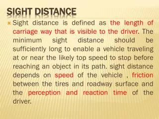
Sight distance is defined as the length of carriage way that is visible to the driver. The minimum sight distance should be sufficiently long to enable a vehicle traveling at or near the likely top speed to stop before reaching an object in its path. sight distance depends on speed of the vehicle , friction between the tires and roadway surface and the perception and reaction time of the driver. Sight Distance
1. Stopping sight distance (SSD): Stopping sight distance is the sum of two distances: a) the distance a vehicle travels after the driver sees an object and before braking ; b)the distance traveled after braking. SSD = d1 + d2 = tv + v2/2gf = 0.278 tv + v2/ 225(fg%)
where: d1 = perception and reaction distance (m.); d2 = breaking distance (m.); v = speed from which the stop is made (km/h) t = perception and reaction time,sec.; f = coeff.of longitudinal friction; g = percent of grade ; recommended as follows: In rural areas = 2.5 sec. In urban areas =1.5 sec.
Minimum sight distance required for safe passing on 2-lane roads consists of 4 elements: (1) d1 : the distance traveled during perception and reaction time to the point of encroachment on the left lane d1 = 0.278 t1 (v-m + a*t1/2) where: t1 : time of preliminary delay. sec.; a : average acceleration rate, km/h/sec.; v : average speed of passing vehicle , km/h; m : difference in speed between passing and passed vehicles, km/h. 2.Passing sight distance (PSD)
(2) d2 : The distance traveled while passing vehicle occupies the left lane d2 = 0.278 v t2 where: t2 : time during which passing vehicle occupies the left lane,sec.; v : average speed of passing vehicle, km/h.
(3) d3 : the distance between the passing vehicle at the end of its maneuver and the opposing vehicle d3 = 30 - 90 m (4) d4 : the distance traveled by an opposing vehicle for 2/3 of the time the passing vehicle occupies the left lane. d4 = 2/3 d2
Road grades may be classified into: a. Road profile grades; b. Ramp grades at grade separations; c. Ditch grade for drainage. CHAPTER 4 HIGHWAY VERTICAL ALIGNMENT
The broad design controls that must be considered as a guide for choice of the grade line, these are: 1.The elevation of existing highways, railways, bridges, waterways and other controlling points that will be crossed by the proposed highway; 2- The ideal grade line is that follows the general topographic conditions or that makes a balance between cut and fill; • a). Road profile grades:
3- Ideal grade line should have long distances between points of intersection with long vertical curves; 4- Two vertical curves in one direction should be separated by a long distance; 5-Suddden ,hidden and unexpected dips should be avoided; 6- Maximum grade should not be exceed the following: 3 % for first class roads of mixed traffic; 5 % for first class roads of passenger cars only; 6-7% for second class and local roads ; 12 % for mountainous or hilly areas. 7- The minimum grade is 0.35 % for surface drainage.
b) Ramp grades: Maximum gradient for up-direction ramp is 7 % Maximum gradient for down-direction ramp is 5 %. c)Ditch grades: The minimum grade for earth ditches ranges from 0.25 -to 0.50% in order to facilitate drainage. Maximum ditch grade should be limited to avoid erosion , this grade should be less than 3% for earth ditches.
Vertical Curves: Vertical curves are used in connecting grade tangents in the profile alignment to provide easy driving and comfort to passengers. These curves are convex when two grades meet on a summit or crest and concave when they meet at a sag. Parabolic curves are generally used for vertical curves because: 1. They are easily to be set and laid out; 2. They enable comfortable transition from one grade to another;
Parabolic curves characteristic: • 1-All distances of the curve are measured on a horizontal plane along the curve, i.e.the distance from P.C. to P.T. is the same whiter it is AVB or ACB or AMB; • 2-All offsets y measured vertically from grade line to the curve; • 3-Offsets are added or subtracted from grade line elevation depending on type of the curve ( summit or sag); • 4-Offsets are symmetrical at both halves of the • curve ; • 5-Rtae of change of grade r = A/L .
Properties of parabolic curves: Vertical curves can be circular , simple parabolic, or cubic parabolic. The simple parabola generally is the preferable curve in highway profile design. From the theory of simple parabolic with equal tangents :
PVI : Point of vertical intersection; where the grade tangents intersect. PVT : Point of vertical tangency; where the curve ends. POVC : Point on vertical curve; applies to any point on the parabola. POVT : Point on vertical tangent; applies to any point on either tangent. g1 : Grade of the tangent on which the PVC is located; measured in percent of slope. g2 : Grade of the tangent on which the PVT is located; measured in percent of slope.
Critical points on vertical curves: It is essential to determine the highest as well as lowest point on the vertical curve to ensure proper drainage or clearance, such as at sag and crests. The critical point is not usually vertically above or below the vertex of the intersecting grade tangents. The distance from the P.C. of the curve to the critical point is derived as follows:
Example : A 5% grade tangent meets a –3% grade tangent at a station 30+0, the elevation of which is equal to 100 m., if the total length of the curve is 160 m.,determine the elevation at each 20 m.
Solution: L=160 m, e=AL/8 =0.08x160/8 = 1.6 m Station at PT= 30+00+0.8 =30+ 80 Station at PC= 30+00-0.8 =29+ 20 Ele.of PC =100-80x0.05 =96.0 m Ele.of PT=100 –80x0.03 =97.6 m Y=4e (x/L)2 = 6.4 (x/L)2 Y1= 6.4 (20/160)2=0.10 m; Y2=6.4 (40/160)2 =0.40 m; Y3=6.4 (60/160)2 =0.90 m; Y4=6.4 (80/160)2 =1.60 m= e