Cache-Oblivious Priority Queue and Graph Algorithm Applications
Cache-Oblivious Priority Queue and Graph Algorithm Applications. Presented by: Raz Berman and Dan Mor. Main Purpose.


Cache-Oblivious Priority Queue and Graph Algorithm Applications
E N D
Presentation Transcript
Cache-Oblivious Priority Queue and Graph Algorithm Applications Presented by: Raz Berman and Dan Mor
Main Purpose The main purpose of the article is developing an optimal cache-oblivious priority queue data structure, supporting insertion, deletion and deletemin operations in a multilevel memory hierarchy. Priority Queues are a critical component in many of the best known cache-aware graph algorithms.
Main Purpose (Cont.) In a cache-oblivious data structure, M (the memory size) and B (the block size) are not used in the description of the structure. The bounds match the bounds of several previously developed cache-aware priority queue data structures, which all rely crucially on knowledge about M and B.
Introduction As the memory systems of modern computers become more complex, it is increasingly important to design algorithms that are sensitive to the structure of memory. One of the essential features of modern memory systems is that they are made up of a hierarchy of several levels of cache, main memory, and disk.
Data Locality In order to amortize the large access time of memory levels far away from the processor, memory systems often transfer data between memory levels in large blocks. Thus it is becoming increasingly important to obtain high data locality in memory access patterns.
The Problem... The standard approach to obtaining good locality is to design algorithms parameterized by several aspects of the memory hierarchy, such as the size of each memory level, and the block size of memory transfers between levels.
The Problem... (Cont.) Unfortunately, this parameterization often leads to complex algorithms that are tuned to particular architectures. As a result, these algorithms are inflexible and not portable.
… and The Solution Recently, the research has aimed at developing memory-hierarchy-sensitive algorithms that avoid any memory-specific parameterization. It has been shown that such cache-oblivious algorithm works optimally on all levels of multilevel memory hierarchy (and not only on a two-level hierarchy, as commonly used for simplicity).
The Solution (Cont.) Cache-oblivious algorithms automatically tune to arbitrary memory architectures. Data locality can be achieved without using the parameters describing the structures of the memory hierarchy.
Memory Hierarchy A typical hierarchy consists of a number of memory levels, with memory level l having size Ml and being composed of Ml/Bl blocks of size Bl. In any memory transfer from level l to l-1, an entire block is moved atomically. Each memory level also has an associated replacement strategy, which is used to decide what block to remove in order to make room for a new block being brought into that level of the hierarchy.
Efficiency Efficiency of an algorithm is measured in terms of the number of block transfers the algorithm performs between two consecutive levels in the memory hierarchy (they are called memory transfers). An algorithm has complete control over placement of blocks in main memory and on disk.
Assumptions • M > B2 (the tall cache assumption). • When an algorithm accesses an element that is not stored in main memory, the relevant block is automatically fetched with a memory transfer. Optimal paging strategy - If the main memory is full, the ideal block in main memory is elected for replacement based on the future characteristics of the algorithm.
Generalization Since an analysis of an algorithm in the two-level model (which was in common use for simulating a multilevel memory hierarchy) holds for any block and main memory size, it holds for any level of the memory hierarchy. As a consequence, if the algorithm is optimal in the two-level model, it is optimal on all levels of the memory hierarchy.
Priority Queue A priority queue maintains a set of elements each with a priority (or key) under the operations insert, delete and deletemin, where a deletemin operation finds and deletes the minimum key element in the queue. Common implementations for a priority queue are heap and B-tree, both support all operations in O(logBN) memory transfers.
The Bounds Sorting N elements requires Θ((N/B)log(M/B)(N/B)) memory transfers. In a B-tree, inset/delmin takes O(logBN) memory transfers, therefore sorting N elements takes O(NlogBN) memory transfers, which is a factor of (BlogBN)/(log(M/B)(N/B)) from optimal. From now on, we will use sort(N) to denote (N/B)log(M/B)(N/B).
The Results The main result is development of an optimal cache-oblivious priority queue, that supports insert, delete and deletemin operations in O((1/B)log(M/B)(N/B)) amortized memory transfers.
Priority Queue – Structure The priority queue data structure consists of Θ(log logN) levels whose sizes vary from N to a constant size c. The size of a level corresponds asymptotically to the number of elements that can be stored within it. For example, the i’th level from above has size . The levels from largest to smallest are N, N2/3, N4/9,…, X9/4, X3/2, X, X2/3, X4/9,…, c9/4, c3/2, c.
Priority Queue – Structure (Cont.) Smaller levels store elements with smaller keys or elements that were more recently inserted. The minimum key element and the most recently inserted element are always in the smallest (lowest) level c. Both insertions and deletions are initially performed on the smallest level and may propagate up through the levels.
Priority Queue - Buffers Elements are stored in a level in a number of buffers, which are also used to transfer elements between levels. Level X consists of one up buffer uX that can store up to X elements, and at most X1/3down buffers, each containing between ½X2/3 and 2X2/3 elements. Thus the maximum capacity of level X is 3X. The size of a down buffer at one level matches the size (up to a constant factor) of the up buffer one level down.
The Invariants Invariant 1: At level X, elements are stored among the down buffers, that is, elements is dix have smaller keys than elements in di+1x, but the elements within dix are unordered. The element with largest key in each down buffer is called a pivot element, and is used to mark the boundaries between the ranges of the keys of elements in down buffers.
The Invariants (Cont.) Invariant 2: At level X, the elements in the down buffers have smaller keys than the elements in the up buffer. Invariant 3: The elements in the down buffers at level X have smaller keys than the elements in the down buffers at the next higher level X3/2.
The Invariants (Cont.) The invariants ensure that the keys of the elements in the down buffers get larger as we go from smaller to larger levels in the structure. At one level, keys of elements in the up buffer are larger than the keys in the down buffers. The keys of an element in an up buffer are unordered relative to the keys of the elements in the down buffer one level up.
Transferring Elements (in general) Up buffers store elements that are “on their way up” – they have yet to be resolved as belonging to a particular down buffer in the next level. Down buffers store elements that are “on their way down” – they have yet to be resolved as belonging to a particular down buffer in the next level down. The element with overall smallest key is in the first down buffer at level c.
Priority Queue - Layout The priority queue is stored in a linear array. The levels are stored consecutively from smallest to largest. Each level occupies 3 times its size, starting with the up buffer (occupying one time its size) followed by the down buffers (occupying two times its size). The total size of the array is O(N).
Operations on Priority Queues We use two general operations – push and pull. Push inserts X elements into level X3/2, and pull removes the X elements with smallest keys from level X3/2, returning them in sorted order. Deletemin (insert) corresponds to pulling (pushing) an element from (to) the smallest level.
Operations (Cont.) Whenever an up buffer in level X overflows, we push the X elements in the buffer one level up, and whenever the down buffers in level X become too empty, we pull X elements from one level up. Both the push and the pull operations maintain the three invariants.
Push To insert X elements into level X3/2, we first sort them using O(1+(X/B)log(M/B)(X/B)) memory transfers and O(Xlog2X) time. Next we distribute them into the X1/2 down buffers of level X3/2. We append an element to the end of the current down buffer, and advance to the next down buffer as soon as we encounter an element with larger key than the key of the pivot of the current down buffer.
Push - Demonstration Level X3/2 .......... Level X
Push (Cont.) Elements with keys larger than the keys of the pivot of the last down buffer are inserted in the up buffer. Level X3/2 .......... Level X
Push (Cont.) Scanning through the elements takes O(1+X/B) memory transfers and O(X) time. We perform one memory transfer for each of the X1/2 down buffers (in the worst case), so the total cost of distributing the elements is O(X/B+X1/2) memory transfers and O(X+X1/2) = O(X) time.
Push - The Elements Distribution If a down buffer runs full (contains 2X elements), we split the buffer into two down buffers each containing X elements, by finding the median of the elements in O(1+X/B) memory transfers and O(X) time and partitioning them in a simple scan in O(X) memory transfers. We assume that the down buffer can be stored out of order, so we just have to update the linked list of buffers.
Push – Splitting a Down Buffer Level X3/2 .......... Level X
Push - The Distribution (Cont.) If the level has already the maximum of X1/2 down buffers before the split, we remove the last down buffer by inserting its elements into the up buffer. Level X3/2 .......... Level X
Push - The Distribution (Cont.) If the up buffer runs full (contains more than X3/2 elements), then all of these elements are pushed into the next level up. Level X3/2 ........ Level X
Push – Total Cost A push of X elements from level X into level X3/2can be performed in O(X1/2+(X/B)log(M/B)(X/B)) memory transfers and O(Xlog2X) time amortized, not counting the cost of any recursive push operations, while maintaining invariants 1-3.
Pull To delete X elements from level X3/2, we first assume that the down buffers at level X3/2 contain at least 3/2*X elements each, so the first three down buffers contain between 3/2*X and 6X elements. We find and remove the X smallest elements by sorting them using O(1+(X/B)log(M/B)(X/B)) memory transfers and O(Xlog2X) time.
Pull - Demonstration Level X3/2 .......... Level X
Pull (Cont.) If the down buffers contain less than 3/2*X elements, we first pull the X3/2 elements with smallest keys from one level up. Level X3/2 ........ Level X
Pull (Cont.) Because these elements do not necessarily have smaller keys than the U elements in the up buffer, we first sort the up buffer, and then we insert the U elements with the largest keys to the up buffer and distribute the remaining elements in the down buffers. Level X3/2 ........ Level X
Pull (Cont.) Afterwards, we can find the X elements with smallest keys as described earlier and remove them. The total cost of a pull of X elements from level X3/2down to level X is O(1+(X/B)log(M/B)(X/B)) memory transfers and O(Xlog2X) time amortized, not counting the cost of any recursive push operations, while maintaining invariants 1-3.
Total Cost #1 The insert (deletemin) is done by performing a push (pull) on the smallest level. This may require recursive pushes (pulls) on higher levels. To maintain that the structure uses Θ(N) space, and has Θ(log logN) levels, it is rebuilt after every N/2 operations (the cost of the rebuilding is worth the effort). It is done by using O((N/B)log(M/B)(N/B)) memory transfers and O(Nlog2N) time, or O((1/B)log(M/B)(N/B)) memory transfers and O(log2N) time per operation.
Total Cost #2 following the previous results, push or pull of X elements to level X use O(X1/2+(X/B)log(M/B)(X/B)) memory transfers. We can reduce this cost to O((X/B)log(M/B)(X/B)) by examining the cost for differently sized levels. In any way, pushing or pulling of X elements is charged to level X.
Total Cost #3 case 1: Pushing or pulling X≥B2 elements into or from level X3/2. In this case, O(X1/2+(X/B)log(M/B)(X/B)) = O((X/B)log(M/B)(X/B)). Proof: O(X1/2+(X/B)log(M/B)(X/B)) = O(B+(B2/B)log(M/B)(B2/B)) = O(B+Blog(M/B)(B2/B)) = O(Blog(M/B)(B2/B)) = O((X/B)log(M/B)(X/B))
Total Cost #4 case 2: Pushing or pulling X<B2 elements into or from level X3/2. In this case, all of the level is kept in memory (since the memory is bigger than B2, because of the tall cache assumption), and therefore all transfer costs associated with this level would be eliminated (we assume that the optimal paging strategy is able to keep the relevant blocks in memory at all times, and thus eliminate these costs).
Total Cost #5 The total cost of an insert or deletemin operation in the sequence of N/2 such operations is memory transfers amortized, and amortized time.
Priority Queue and Graph Algorithms We will now show how the cache-oblivious priority-queue can be used to develop several cache-oblivious graph algorithms – list ranking, BFS, DFS and minimal spanning tree.
List Ranking In this problem we have a linked list with V nodes, stored as an unordered sequence, each containing the position of the next node in the list (an edge). Each edge has a weight and the goal is to find for each node v the sum of the weights of edges from v to the end of the list. For example, if all the weights are 1, then the goal is to determine the number of edges from v to the end of the list (called the rank of v).
List Ranking – Main Idea An independent set of Θ(V) nodes is found, nodes in the independent set are “bridging out”, the remaining list is recursively ranked, and finally the contracted nodes are reintegrated into the list, while computing their ranks.