AP Statistics Topic 2
AP Statistics Topic 2. ‘Intro to Statistics and Data Analysis’ by POD will be our primary source In Topic 1 we collected and produced data In Topic 2 we will learn to summarize univariate data Chapter 3 Graphical Methods for Displaying Data Chapter 4 Numerical Methods for Describing Data.

AP Statistics Topic 2
E N D
Presentation Transcript
AP StatisticsTopic 2 • ‘Intro to Statistics and Data Analysis’ by POD will be our primary source • In Topic 1 we collected and produced data • In Topic 2 we will learn to summarize univariate data • Chapter 3 • Graphical Methods for Displaying Data • Chapter 4 • Numerical Methods for Describing Data
Some Vocabulary • Population • The entire collection of individuals or objects we are interested in • Sample • A subset representative of the population • It’s from this sample that we make conclusions about the population – important that the sample is representative • Why only study a sample?
Can’t underestimate variability • If we are studying a process or population by collecting and analyzing data from a sample from this process/population, we would expect to see a certain amount of variability • How much variability or differences in the measurements is normal and at what point do you suspect an underlying reason other than natural variability? • Consider the semi-conductor manufacturing process. Statistics used in quality control. • The ability to recognize unusual values in the presence of variability is the essence of statistical methods we’ll studying in this course.
What is data? • Individuals or objects in any particular population possess many characteristics • Ex. Characteristics of students at LJCD might include the type of car they drive, the number of textbooks they have, the color of their hair, their height • Variable • Any characteristic that can change from person to person is referred to as a variable • Data • Data are the results of making observations on one or more characteristics of the individuals from the population of interest
A few more comments about data • When we measure data on a single characteristic – our data in univariate • Heights of seniors at LJCD • When we measure data on two attributes – bivariate • Cholesterol level and body weight of adult males • More than two attributes -- multivariate
Types of Data • Categorical • A qualitative observation about an individual or object • Ex. Hair color, airline flown, preferred activity • Numerical • Observation on individual or object is a number • Ex. Height, SAT score, time person stands in line
Two Types of Numerical Data • Discrete • Possible data values are isolated points on the number line • Rule of thumb – counts of things • Number of people standing in line at Von’s • Continuous • Possible values fall into an interval on the number line • Rule of thumb – measurements • Height of girls in our class, gas mileage of cars
Graphical Methods for Describing Data • When we study a process or a population we often collect data. • After collecting and tabulating the data, we want to do some simple analysis. We want to describe what we see before we study any relationships and look to make judgments about the population from which the data was drawn. • First we graph the data and then we generate the appropriate numerical summaries.
Let’s say … • We’re interested in the amount of caffeine in popular soft drinks. • While the data in this table is nicely organized, it’s difficult to make any sense of what the data might be telling us. • FDA Table
Displaying Categorical Data • Today we’ll look at graphical displays of categorical data • Provide an example of a categorical variable • Specifically • Frequency Distribution Table & Relative Frequency Distribution Table • Bar Chart • Pie Chart
Frequency Distribution Table • A table that displays variable categories and the associated frequencies or relative frequencies • Soft Drink Sales Table
Bar Charts • A Bar Chart is a graph of a frequency distribution table • Horizontal line with category labels • Vertical line with scale using either frequency or relative frequency • Place a rectangle above each category label. Height determined by freq or rel freq. All widths should be the same. • What to look for: frequently and infrequently occurring categories
Comparative Bar Chart • Variation of the Bar Chart • Above each category label are bars based on frequency or relative frequency of two characteristics for each category
Pie Charts • A Pie Chart is a graphical representation of a frequency distribution table • Used for categorical data with relatively few categories • Draw a circle to represent the entire data set • Each slice size: • What to look for: categories that form large and small proportions of the data
Graphical Display of Numerical Data • A simple display with a small amount of data – the dotplot • Consider the range of data • You may round your data • ‘stack the BB’s’ • Description of your data
So far ….. • We talked about some of the very basic vocabulary of statistics • Population • Sample • Data • Numerical or categorical • Numerical data • Discrete or Continuous • Variability • Distribution of data • Since data varies, we’re interested in its distribution • What are the values and how often do they occur • Graphical displays of categorical data • Frequency Distribution Tables • Pie Charts • Bar Charts • Graphical display of numerical data • Dotplot
Displaying Numerical Data • When we displayed categorical data, we generally were interested in the question ‘How often does a certain type of response occur?’/’What proportion of the data falls into various categories?’ • When we study numerical data, the types of questions include • What is a typical value? • Is the data concentrated around a particular value or is it spread out? • Is there one value that occurs most frequently or more than one value? • Is the data symmetric or skewed? • Are there gaps on the data? • Are there any values that are unusual?
The Displays we’ll study are … • Dot plots • Stem and Leaf Displays • Frequency Distribution Tables • Histograms • Time Series Displays • Ogive (Cumulative Relative Frequency Plot)
Dot Plots • Simplest way to display numerical data • Small data sets • Data is discrete • How to construct: • Draw a horizontal line with an appropriate scale • Locate each value in the data set along the horizontal line and represent it with a dot. • ‘Stack the BB’s’ • Indicate units someplace in the display
What we are looking for … • Typical value • Spread of the data • Shape • Gaps and/or clusters • Outliers • Number and location of peaks
Let’s look at an example • Gas Mileage for ’02 midsize cars • Comment on the features of this dotplot
Stem and Leaf Display • Another simple way to display numerical data • Small to moderate data sets • Data is discrete • How to construct: • Select one or more leading digits for stem values • List the possible stem values either vertically or horizontally • Record the leaf for each data value beside/above the appropriate stem value • Indicate units someplace in the display
Let’s look at an example • San Diego County 6th grade test scores – single digit stem • Sales Prices of homes – two digit stems • FDA Study of Caffeine – truncated • San Diego County 6th grade test scores -- comparative • Comment on the features • What’s also nice about Dot Plots and Stem and Leaf Displays is you can reconstruct all of your data.
Consider this… • For this data, which display is better and why? • Cheddar Cheese data set
Population vs Sample Variability Data Categorical and Numerical Discrete and Continuous Graphical Displays Bar Charts and Pie Charts Doptlots Stem and Leaf Histograms Descriptions 6 Categories Typical value Variability Peaks Gaps or Clusters Shape Unusual Values Summary
Frequency Distribution Tables and Histograms • Dot Plots and Stem and Leaf Displays work well with small to moderate sets of data • For larger sets of data, two displays that work well are the Frequency Distribution Table and the Histogram • Both of these displays are suited for both discrete and continuous data
Frequency Distribution Tables • Fairly simple to make • For discrete data • List the possible values the the data can take on • Much like the categories for qualitative data • If there are many possible values you can group values together (classes) • For continuous data • Break the interval of values into classes of equal width • List the frequency of occurrence of each value or frequency of occurrence in each class • You can also determine the relative frequency • Rule of thumb for number of classes is • ‘Hits per Game’ data for a discrete example • ‘Water Quality’ data for a continuous example
Histograms • Use the Frequency Distribution to organize your data • Draw a horizontal scale and mark the possible values • Above each value or class, draw a rectangle -- centered on that value for discrete data. The height is determined by the frequency or relative frequency of that discrete value or frequency within that interval • The widths of each rectangle are the same and their sides touch • Make histograms for the previous examples • Comment on the same 6 features
Histogram Shapes • Number of peaks – modes • Shape – symmetric or skewed • Upper tail and Lower tail • Light tailed and Heavy tailed • Relative to the normal curve • Positively and Negatively skewed • Skewed left and Skewed right
Cumulative Relative Frequencies • Relative frequency table tells us what proportion of the data falls in a particular class • We may be interested in the proportion of data that falls below or above a particular value. • We can get this info from a Cumulative Relative Frequency Table • Percentile: the pth percentile of a distribution is the value such that p% of the observations fall at or below it. • How to create this table: • Sum the relative frequencies for each class • EX. July Home Resale Prices
Do Histograms Resemble the Population Histogram ? • Sample data is collected from a population of interest in order to make inferences about that population. • Samples should be representative of the population. • It follows that a sample histogram should therefore resemble the population histogram.
Examples • First, 3 samples from a Normal Population • Second, 3 samples from a skewed population • We’ll use the 2001 San Diego July Resale Prices • List 2 is the population of 85 Resale Prices • List 3 is a random sample of 10 • List 4 is a random sample of 30 • Compare the histograms
Time Series Plots • One final graphic display of data is the Time Series plot • We typically look for observations vs time • Ex. DJIA • We’re interested in • Patterns • Deviations from a pattern • Trends
Chapter 4Numerical Methods for Describing Data • In Chapter 3 of the text we studied graphical displays of data. The purpose being to get a general sense of the data guided by the 6 features • In Chapter 4 we’ll study numerical summary methods that give us a more precise description of center and spread.
Describing the Center of a Data Set • The two most popular measures of the center of a data set are the mean and the median. • The mean is simply the arithmetic average • The median is the middle value of the data set • The middle value when you have an odd number of data points • The average of the two middle observations when you have an even number of data points
Terminology • We’ve already distinguished between population and sample • Population statistics are represented by the Greek letters • Sample statistics are represented by the Roman letters • Sample statistics are used as estimates for population statistics
Let’s Compare the Mean and Median • For symmetric data, the mean equals (or is very close to) the median • For skewed data, the mean and median are different • The mean is affected by unusual values/outliers • The median is unaffected by outliers – we use the term ‘resistant’ to describe a statistic that is unaffected by outliers • Let’s look at two data sets • Inspect histograms • Calculate mean and median
Trimmed Mean • The extreme sensitivity of the mean to even a single outlier and the median’s complete insensitivity to many outliers was cause for statisticians to develop a statistic that is a compromise of the two • This statistic is the trimmed mean. • Definition: A trimmed mean is computed by first ordering the data from smallest to largest, deleting a selected number of values from each end and then averaging the remaining values. The trimming percentage is the percentage of values selected from each end of the ordered list --
Numerical Summary for Categorical Data • The numerical summary quantities for categorical data are the relative frequencies for the various categories • We call these relative frequencies ‘proportions’ – and similar to means and medians – we have sample proportion (p) and population proportion ( ) • An example
Describing Variability in Data • Yesterday we discussed different measures of center for a sample of numerical data • Reporting only the measure of center gives only partial information • It’s also important to describe how the data is spread about the center
Describing Variability • Consider this display of 3 sets of data • Measure of center for each? • Most variable? • Least variable? • How does the variability compare as you move from 1 to 2 to 3? Why? • A measure of variability gives useful info and more insight
Measures of Variability • Range • Difference between min and max value • Not a good measure – see sets 1 and 2 • Variance/Standard Deviation • Measures extent to which data varies about the mean • Interquartile Range • Measure of variability associated with the median
Variance/Standard Deviation • The most common measure • Associated with the mean best used to describe symmetric data • A measure that describes the deviation about the mean
Deviations from the Mean • Consider this as a measure for variability about the mean • Does this seem reasonable? • Consider this data – Bobby Bonds HR totals through 2001 over his career • 16 19 24 25 25 33 33 34 37 37 37 40 42 46 49 73
Deviation about the Mean • Find • Now find • The point is • Is this a good measure? Why not?
Squared Deviations about the Mean • This measure won’t allow positive and negative values to cancel • Divide by n and we have the average squared deviation from the mean • In statistics we divide by n-1 and call our value sample variance –
Why divide by n-1? • Empirically, sample variance is a better estimator for population variance when you divide by n-1 • There’s another statistical explanation referred to degrees of freedom
Sample Standard Deviation • The square root of the variance is the sample standard deviation – • We use standard deviation because it gives a measure in the same units as our data