Simple Regression Relationships: Interpretation & Computation
This lecture covers interpreting regression output, parameter estimates, computing R-square, standard error, and more. Learn how to analyze the significance of the relationship between variables and the impact on predictions.

Simple Regression Relationships: Interpretation & Computation
E N D
Presentation Transcript
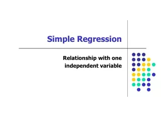
Simple Regression Relationship with one independent variable
Lecture Objectives • You should be able to interpret Regression Output. Specifically, • Interpret Significance of relationship (Sig. F) • The parameter estimates (write and use the model) • Compute/interpret R-square, Standard Error (ANOVA table)
ŷ = b0 + b1X є Dependent variable (y) b1 = slope = ∆y/ ∆x b0 (y intercept) Independent variable (x) Basic Equation The straight line represents the linear relationship between y and x.
Understanding the equation What is the equation of this line?
Variation from mean (Total Variation) Mean Y Dependent variable (y) Independent variable (x) Total Variation Sum of Squares (SST) What if there were no information on X (and hence no regression)? There would only be the y axis (green dots showing y values). The best forecast for Y would then simply be the mean of Y. Total Error in the forecasts would be the total variation from the mean.
Sum of Squares Total (SST) Computation In computing SST, the variable X is irrelevant. This computation tells us the total squared deviation from the mean for y.
Total Variation Residual Error (unexplained) Explained by regression Dependent variable (y) Mean Y Independent variable (x) Error after Regression Information about x gives us the regression model, which does a better job of predicting y than simply the mean of y. Thus some of the total variation in y is explained away by x, leaving some unexplained residual error.
The Regression Sum of Squares Some of the total variation in y is explained by the regression, while the residual is the error in prediction even after regression. Sum of squares Total = Sum of squaresexplained by regression + Sum of squares oferror still left after regression. SST = SSR + SSE or, SSR = SST - SSE
R-square The proportion of variation in y that is explained by the regression model is called R2. R2 = SSR/SST = (SST-SSE)/SST Forthe shoe size example, R2 = (48.8077 – 17.6879)/48.8077 = 0.6376. R2 ranges from 0 to 1, with a 1 indicating a perfect relationship between x and y.
Mean Squared Error MSR = SSR/dfregression MSE = SSE/dferror df is the degrees of freedom For regression, df = k = # of ind. variables For error, df = n-k-1 Degrees of freedom for error refers to the number of observations from the sample that could have contributed to the overall error.
Standard Error Standard Error (SE) = √MSE Standard Error is a measure of how well the model will be able to predict y. It can be used to construct a confidence interval for the prediction.
Summary Output & ANOVA = SSR/SST = 31.1/48.8 = √MSE = √ 1.608 p-value for regression =MSR/MSE =31.1/1.6
The Hypothesis for Regression H0: β1 = β2= β3 = … = 0 Ha: At least one of the βs is not 0 If all βs are 0, then it implies that y is not related to any of the x variables. Thus the alternate we try to prove is that there is in fact a relationship. The Significance F is the p-value for such a test.