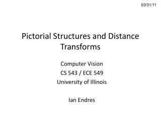
Pictorial Structures and Distance Transforms
520 likes | 684 Vues
This lecture discusses advanced methodologies for object detection focusing on Cars, Faces, and Cats using techniques such as Pictorial Structures and Distance Transforms. It explores statistical template modeling, feature extraction related to bounding box coordinates, and the optimization of detection models through dynamic programming. The course analyzes articulated parts, the interplay of appearance and spatial configurations, and applies deformable part models in detecting objects. The fundamental concepts are contextualized with examples from datasets like Caltech-101 and Caltech-256, making it a comprehensive guide for understanding modern object detection.

Pictorial Structures and Distance Transforms
E N D
Presentation Transcript
03/31/11 Pictorial Structures and Distance Transforms Computer Vision CS 543 / ECE 549 University of Illinois Ian Endres
Goal: Detect all instances of objects Cars Faces Cats
Object model: last class • Statistical Template in Bounding Box • Object is some (x,y,w,h) in image • Features defined wrt bounding box coordinates Image Template Visualization Images from Felzenszwalb
Last class: statistical template • Object model = log linear model of parts at fixed positions ? +3 +2 -2 -1 -2.5 = -0.5 > 7.5 Non-object ? +4 +1 +0.5 +3 +0.5 = 10.5 > 7.5 Object
When are statistical templates useful? Caltech 101 Average Object Images
Deformable objects Images from Caltech-256 Slide Credit: Duan Tran
Deformable objects Images from D. Ramanan’s dataset Slide Credit: Duan Tran
Object models: this class • Articulated parts model • Object is configuration of parts • Each part is detectable Images from Felzenszwalb
Parts-based Models Define object by collection of parts modeled by • Appearance • Spatial configuration Slide credit: Rob Fergus
How to model spatial relations? • Star-shaped model Part Part Part Root Part Part
How to model spatial relations? • Star-shaped model Part = Part X Part X Root ≈ Part Part X
How to model spatial relations? • Tree-shaped model
How to model spatial relations? • Many others... O(N6) O(N2) O(N3) O(N2) Fergus et al. ’03 Fei-Fei et al. ‘03 Leibe et al. ’04, ‘08Crandall et al. ‘05 Fergus et al. ’05 Crandall et al. ‘05 Felzenszwalb & Huttenlocher ‘05 Csurka ’04 Vasconcelos ‘00 Bouchard & Triggs ‘05 Carneiro & Lowe ‘06 from [Carneiro & Lowe, ECCV’06]
Today’s class • Tree-shaped model • Example: Pictorial structures • FelzenszwalbHuttenlocher 2005 • Optimization with Dynamic Programming • Distance Transforms
Pictorial Structures Model Part = oriented rectangle Spatial model = relative size/orientation Felzenszwalb and Huttenlocher 2005
Part representation • Background subtraction
Pictorial Structures Model Geometry likelihood Appearance likelihood
Modeling the Appearance • Any appearance model could be used • HOG Templates, etc. • Here: rectangles fit to background subtracted binary map • Train a detector for each part independently Geometry likelihood Appearance likelihood
Pictorial Structures Model Minimize Energy (-log of the likelihood): Appearance Cost Geometry Cost
Optimization – Brute Force Appearance Cost Deformation Cost H T F
Optimization H T F
Optimization - Complexity Each part can take N locations ? For all lT? H Overall? (for K parts) T F
Distance Transform • For each pixel p, how far away is the nearest pixel q of set S • G is often the set of edge pixels G: black pixels p1 q1 q2 p2
Computing the Distance Transform • 1-Dimension
Computing the Distance Transform • Extending to N-Dimensions • Savings can be extended from 1-D to N-D cases if deformation cost is separable:
Distance Transform - Applications • Set distances – e.g. Hausdorff Distance • Image processing – e.g. Blurring • Robotics – Motion Planning • Alignment • Edge images • Motion tracks • Audio warping • Deformable Part Models (of course!)
Generalized Distance Transform • Original form: • General form: • m(q): arbitrary function sampled at discrete points • For each p, find a nearby q with small m(q) • For original DT: • For part models: • For some deformation costs,
How do we do it? • Key idea: Construct lower “envelope” of data • Given envelope, compute f(p) in O(N) time • Goal: Compute envelope in O(N) time
Computing the Lower Envelope • Key idea: Keep track of intersection points • fi(x), fj(x) only intersect once (let i<j) Start(1) = -Inf End(1) = Inf
Computing the Lower Envelope • Key idea: Keep track of intersection points • fi(x), fj(x) only intersect once (let i<j) Start(1) = -Inf End(1) = 3 Start(2) = 3 End(2) = Inf X
Computing the Lower Envelope • Key idea: Keep track of intersection points • fi(x), fj(x) only intersect once (let i<j) Start(1) = -Inf End(1) = 3 Start(2) = 3 End(2) = 4 Start(3) = 4 End(3) = Inf X
Computing the Lower Envelope • Key idea: Keep track of intersection points • fi(x), fj(x) only intersect once (let i<j) Start(1) = -Inf End(1) = 3 Start(2) = 3 End(2) = 4 Start(3) = 4 End(3) = Inf X
Computing the Lower Envelope • Key idea: Keep track of intersection points • fi(x), fj(x) only intersect once (let i<j) Start(1) = -Inf End(1) = 3 Start(2) = 3 End(2) = 4 Start(3) = [] End(3) = [] Start(4) = 4 End(4) = Inf X
Computing the Lower Envelope • Key idea: Keep track of intersection points • fi(x), fj(x) only intersect once (let i<j) Start(1) = -Inf End(1) = 3 Start(2) = 3 End(2) = 4 Start(3) = [] End(3) = [] Start(4) = 4 End(4) = Inf X
Computing the Lower Envelope • Key idea: Keep track of intersection points • fi(x), fj(x) only intersect once (let i<j) Start(1) = -Inf End(1) = 3 Start(2) = 3 End(2) = 4 Start(3) = [] End(3) = [] Start(4) = 4 End(4) = Inf X
Computing the Lower Envelope • Key idea: Keep track of intersection points • fi(x), fj(x) only intersect once (let i<j) Start(1) = -Inf End(1) = 3 Start(2) = [] End(2) = [] Start(3) = [] End(3) = [] Start(4) = 3 End(4) = Inf X
Computing the Lower Envelope • Key idea: Keep track of intersection points • fi(x), fj(x) only intersect once (let i<j) Start(1) = -Inf End(1) = 2.6 Start(2) = [] End(2) = [] Start(3) = [] End(3) = [] Start(4) = 2.6 End(4) = Inf X
Computing the Lower Envelope • Key idea: Keep track of intersection points • fi(x), fj(x) only intersect once (let i<j) Start(1) = -Inf End(1) = 2.6 Start(2) = [] End(2) = [] Start(3) = [] End(3) = [] Start(4) = 2.6 End(4) = 3.5 Start(5) = 3.5 End(5) = Inf X
Is This O(N)? • Yes! • N parabolas are added • For each addition, may remove up to O(N) parabolas • But, each parabola can only be deleted once • Thus, O(N) additions, and at most O(N) deletions
What distances can we use? • Quadratic (with linear shift) • Abs. diff • Min-composition • Bounded (Requires extra bookkeeping)
Back to the Pictorial structures model Problem: May need to infer more than one configuration • May be more than one object • Report scores for every root position, apply NMS • Optimal solution may be incorrect • Sampling • Sample root node, then each node given parent, until all parts are sampled
Sample poses from likelihood and choose best match with Chamfer distance to map
Results for person matching - Mistakes • Ambiguous Background subtracted image
Recently enhanced pictorial structures BMVC 2009