Hierarchical Models and Variance Components
390 likes | 526 Vues
Hierarchical Models and Variance Components. Will Penny. Wellcome Department of Imaging Neuroscience, University College London, UK. SPM Course, London, May 2003. Outline. Random Effects Analysis Summary statistic approach (t-tests @ 2 nd level) General Framework

Hierarchical Models and Variance Components
E N D
Presentation Transcript
Hierarchical Models and Variance Components Will Penny Wellcome Department of Imaging Neuroscience, University College London, UK SPM Course, London, May 2003
Outline • Random Effects Analysis Summary statistic approach (t-tests @ 2nd level) • General Framework Multiple variance components and Hierarchical models • Multiple variance components F-tests and conjunctions @2nd level Modelling fMRI serial correlation @1st level • Hierarchical models for Bayesian Inference SPMs versus PPMs
Outline • Random Effects Analysis Summary statistic approach (t-tests @ 2nd level) • General Framework Multiple variance components and Hierarchical models • Multiple variance components F-tests and conjunctions @2nd level Modelling fMRI serial correlation @1st level • Hierarchical models for Bayesian Inference SPMs versus PPMs
^ ^ ^ ^ ^ 11 12 1 2 ^ ^ ^ ^ 2 12 1 11 Random Effects Analysis:Summary-Statistic Approach 1st Level 2nd Level DataDesign MatrixContrast Images SPM(t) One-sample t-test @2nd level
Validity of approach • Gold Standard approach is EM – see later – estimates population mean effect as MEANEM the variance of this estimate as VAREM • For N subjects, n scans per subject and equal within-subject variance we have VAREM = Var-between/N + Var-within/Nn • In this case, the SS approach gives the same results, on average: Avg[a] = MEANEM Avg[Var(a)] =VAREM • In other cases, with N~12, and typical ratios of between-subject to within-subject variance found in fMRI, the SS approach will give very similar results to EM. ^ ^
Example: Multi-session study of auditory processing SS results EM results Friston et al. (2003) Mixed effects and fMRI studies, Submitted.
Two populations Estimated population means Contrast images Two-sample t-test @2nd level
Outline • Random Effects Analysis Summary statistic approach (t-tests @ 2nd level) • General Framework Multiple variance components and Hierarchical models • Multiple variance components F-tests and conjunctions @2nd level Modelling fMRI serial correlation @1st level • Hierarchical models for Bayesian Inference SPMs versus PPMs
The General Linear Model y = X + e N 1 N L L 1 N 1 Error covariance N 2 Basic Assumptions • Identity • Independence N We assume ‘sphericity’
Multiple variance components y = X + e N 1 N L L 1 N 1 Error covariance N Errors can now have different variances and there can be correlations N We allow for ‘nonsphericity’
Non-Sphericity Error Covariance • Errors are independent but not identical • Errors are not independent and not identical
General Framework Multiple variance components at each level Hierarchical Models With hierarchical models we can define priors and make Bayesian inferences. If we know the variance components we can compute the distributions over the parameters at each level.
( ) - 1 - = T 1 C X C X e q E-Step y - h = T 1 C X C y e q q y y for i and j { = - h r y X q y M-Step - - - - - = - - 1 T 1 1 T 1 1 g tr { Q C } r C Q C r tr { C X C Q C X } e e e e e q i i i i y - - = } 1 1 J tr { Q C Q C } e e ij j i - l = l - 1 J g å = + l C C Q e q k k Estimation EM algorithm Friston, K. et al. (2002), Neuroimage
Algorithm Equivalence Parametric Empirical Bayes (PEB) Hierarchical model EM=PEB=ReML Restricted Maximimum Likelihood (ReML) Single-level model
Outline • Random Effects Analysis Summary statistic approach (t-tests @ 2nd level) • General Framework Multiple variance components and Hierarchical models • Multiple variance components F-tests and conjunctions @2nd level Modelling fMRI serial correlation @1st level • Hierarchical models for Bayesian Inference SPMs versus PPMs
Non-Sphericity Error Covariance • Errors are independent but not identical • Errors are not independent and not identical
Non-Sphericity Error can be Independent but Non-Identical when… 1) One parameter but from different groups e.g. patients and control groups 2) One parameter but design matrices differ across subjects e.g. subsequent memory effect
Non-Sphericity • Error can be Non-Independent and Non-Identical when… • 1) Several parameters per subject • e.g. Repeated Measurement design • 2) Conjunction over several parameters • e.g.Common brain activity for different cognitive processes • 3) Complete characterization of the hemodynamic response • e.g. F-test combining HRF, temporal derivative and dispersion regressors
Example I U. Noppeney et al. Stimuli:Auditory Presentation (SOA = 4 secs) of (i) words and (ii) words spoken backwards Subjects: (i) 12 control subjects (ii) 11 blind subjects jump touch koob “click” Scanning: fMRI, 250 scans per subject, block design Q. What are the regions that activate for real words relative to reverse words in both blind and control groups?
Independent but Non-Identical Error 1st Level Controls Blinds 2nd Level Controls and Blinds Conjunction between the 2 groups
Example 2 U. Noppeney et al. Stimuli:Auditory Presentation (SOA = 4 secs) of words Subjects: (i) 12 control subjects motion sound visual action jump touch “jump” “click” “pink” “turn” “click” Scanning: fMRI, 250 scans per subject, block design Q. What regions are affected by the semantic content of the words ?
Non-Independent and Non-Identical Error 1st Leve visual sound hand motion ? = ? = ? = 2nd Level F-test
Example III U. Noppeney et al. Stimuli:(i) Sentences presented visually (ii) False fonts (symbols) Some of the sentences are syntactically primed Scanning: fMRI, 250 scans per subject, block design Q. Which brain regions of the “sentence reading system” are affected by Priming?
Non-Independent and Non-Identical Error 1st Level Sentence > Symbols No-Priming>Priming Orthogonal contrasts 2nd Level Conjunction of 2 contrasts Left Anterior Temporal
Example IV Modelling serial correlation in fMRI time series Model errors for each subject as AR(1) + white noise.
Outline • Random Effects Analysis Summary statistic approach (t-tests @ 2nd level) • General Framework Multiple variance components and Hierarchical models • Multiple variance components F-tests and conjunctions @2nd level Modelling fMRI serial correlation @1st level • Hierarchical models for Bayesian Inference SPMs versus PPMs
Example 2:Univariate model Likelihood and Prior Posterior Relative Precision Weighting
Example 2:Univariate model Likelihood and Prior AIM: Make inferences based on posterior distribution Similar expressions exist for posterior distributions in multivariate models Posterior But how do we compute the variance components or ‘hyperparameters’ ?
( ) - 1 - = T 1 C X C X e q E-Step y - h = T 1 C X C y e q q y y for i and j { = - h r y X q y M-Step - - - - - = - - 1 T 1 1 T 1 1 g tr { Q C } r C Q C r tr { C X C Q C X } e e e e e q i i i i y - - = } 1 1 J tr { Q C Q C } e e ij j i - l = l - 1 J g å = + l C C Q e q k k Estimation EM algorithm Friston, K. et al. (2002), Neuroimage
Estimating mean and variance Maximum Likelihood (ML), maximises p(Y|m,b) Expectation-Maximisation (EM), maximises for ‘vague’ prior on m
Estimating mean and variance For a prior on m with prior mean 0 and prior precision a Expectation-Maximisation (EM) gives where Larger a more shrinkage
Estimating mean and variance at multiple voxels For a prior on m over voxels with prior mean 0 and prior precision a Expectation-Maximisation (EM) gives at voxel i=1..V, scan n=1..N where Prior precision can be estimated from data. If mean activation over all voxels is 0 then these EM estimates are more accurate than ML
The Interface PEB Parameters and Hyperparameters WLS Parameters, REML Hyperparameters Shrinkage priors No Priors
Bayesian Inference 1st level = within-voxel Likelihood Shrinkage Prior In the absence of evidence to the contrary parameters will shrink to zero 2nd level = between-voxels
Bayesian Inference: Posterior Probability Maps PPMs Posterior Likelihood Prior SPMs
SPMs and PPMs PPMs: Show activations of a given size SPMs: show voxels with non-zero activations
PPMs Advantages Disadvantages Use of shrinkage priors over voxels is computationally demanding Utility of Bayesian approach is yet to be established One can infer a cause DID NOT elicit a response SPMs conflate effect-size and effect-variability P-values don’t change with search volume For reasonable thresholds have intrinsically high specificity
Summary • Random Effects Analysis Summary statistic approach (t-tests @ 2nd level) • Multiple variance components F-tests and conjunctions @2nd level Modelling fMRI serial correlation @1st level • Hierarchical models for Bayesian Inference SPMs versus PPMs • General Framework Multiple variance components and Hierarchical models