3.7 Diffraction
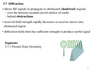
3.7 Diffraction. allows RF signals to propagate to obstructed ( shadowed ) regions - over the horizon (around curved surface of earth) - behind obstructions received field strength rapidly decreases as receiver moves into obstructed region

3.7 Diffraction
E N D
Presentation Transcript
3.7 Diffraction • allows RF signals to propagate to obstructed (shadowed) regions • - over the horizon (around curved surface of earth) • - behind obstructions • received field strength rapidly decreases as receiver moves into • obstructed region • diffraction field often has sufficient strength to produce useful signal Segments 3.7.1 Fresnel Zone Geometry
slit knife edge • Huygen’s Principal • all points on a wavefront can be considered as point sources for • producing 2ndry wavelets • 2ndry wavelets combine to produce new wavefront in the direction • of propagation • diffraction arises from propagation of 2ndry wavefront into • shadowed area • field strength of diffracted wave in shadow region = electric field • components of all 2ndry wavelets in the space around the obstacle
d = d1+ d2, where , di = h d = + – (d1+d2) TX RX d1 d2 ht hobs hr Knife Edge Diffraction Geometry for ht = hr • 3.7.1 Fresnel Zone Geometry • consider a transmitter-receiver pair in free space • let obstruction of effective height h &width protrude to page • - distance from transmitter = d1 • - distance from receiver = d2 • - LOS distance between transmitter & receiver = d = d1+d2 Excess Path Length = difference between direct path & diffracted path = d – (d1+d2)
3.54 3.55 = = h h’ TX d1 d2 RX hobs ht hr Knife Edge Diffraction Geometry ht > hr Assume h << d1 , h <<d2 and h >> then by substitution and Taylor Series Approximation Phase Difference between two paths given as
tan(x) TX hobs-hr ht-hr RX d1 d2 x tan = tan = x = 0.4 rad tan(x) = 0.423 (0.4 rad ≈ 23o ) Equivalent Knife Edge Diffraction Geometry with hrsubtracted from all other heights 180- when tan x x = +
v = (3.56) when is inunits of radians is given as = (3.57) Eqn 3.55 for is often normalized using the dimensionless Fresnel-Kirchoffdiffraction parameter, v • from equations 3.54-3.57 , the phase difference, between LOS & diffracted path is function of • obstruction’s height & position • transmitters & receiversheight & position • simplify geometry by reducing all heights to minimum height
d λ/2 + d λ + d 1.5λ + d • (1) Fresnel Zones • used to describe diffraction loss as a function of path difference, • around an obstruction • represents successive regions between transmitter and receiver • nthregion = region where path length of secondary waves is n/2 • greater than total LOS path length • regions form a series of ellipsoids with foci at Tx & Rx at 1 GHz λ = 0.3m
R = T slice an ellipsoid with a plane yields circle with radius rn given as h = rn = then Kirchoffdiffraction parameter is given as v = = thus for given rnvdefines an ellipsoid with constant = n/2 • Construct circles on the axis of Tx-Rx such that = n/2, for given integer n • radii of circles depends on location of normal plane between Tx and Rx • given n, the set of points where = n/2 defines a family of ellipsoids • assuming d1,d2 >> rn
nthFresnel Zone is volume enclosed by ellipsoid defined for n andis defined as relative to LOS path • 1st Fresnel Zone is volume enclosed by ellipsoid defined forn = 1 Phase Difference, pertaining to nthFresnel Zone is ≤ Δ≤ (n-1)≤ ≤ n • contribution to the electric field at Rx from successive Fresnel Zones • tend to be in phase opposition destructive interference • generally must keep 1st Fresnel Zone unblocked to obtain free space • transmission conditions
d d2 d1 • destructive interference • = /2 • d = /2 + d1+d2 Tx Rx • constructive interference: • d = + d1+d2 • = For 2nd Fresnel Zone • For 1st Fresnel Zone, at a distance d1from Tx & d2 from Rx • diffracted wave will have a path length of d
Q R h d2 O T d1 • Fresnel Zones • slice the ellipsoids with a transparent plane between transmitter & • receiver – obtain series of concentric circles • circles represent loci of2ndry wavelets that propagate to receiver • such that total path length increases by /2 for each successive circle • effectively produces alternativelyconstructive &destructive • interference to received signal • If an obstruction were present, it could block some of the Fresnel • zones
n =n/2 1 /2 2 rn = (3.58) 3 3/2 Excess Total Path Length, for each ray passing through nth circle Rx Tx Assuming, d1& d2 >> rn radius of nth Fresnel Zone can be given in terms of n, d1,d2, • radii of concentric circles depends on location between Tx & Rx • - maximum radii at d1 = d2 (midpoint), becomes smaller as plane • moves towards receiver or transmitter • - shadowing is sensitive to obstruction’s position and frequency
(2) Diffraction Loss caused by blockage of 2ndry (diffracted) waves • partial energy from 2ndry waves is diffracted around an obstacle • obstruction blocks energy from some of the Fresnel zones • only portion of transmitted energy reaches receiver • received energy = vector sum of contributions from all unobstructed • Fresnel zones • depends on geometry of obstruction • Fresnel Zones indicate phase of secondary (diffracted) E-field • Obstacles may block transmission paths – causing diffraction loss • construct family of ellipsoids between TX & RX to represent • Fresnel zones • join all points for which excess path delay is multiple of /2 • compare geometry of obstacle with Fresnel zones to determine • diffraction loss (or gain)
Rx Tx Diffraction Losses • Place ideal, perfectly straight screen between Tx and Rx • (i) if top of screen is well below LOS path screen will have little effect • - the Electric field at Rx = ELOS (free space value) • (ii) as screen height increases E will vary up & down as screen blocks more • Fresnel zones below LOS path • amplitude of oscillation increases until just in line with Tx and Rx • field strength = ½ of unobstructed field strength
e.g. v = excess path length /2 3/2 RX TX h d1 d2 and v are positive, thus h is positive • Fresnel zones: ellipsoids with foci at transmit & receive antenna • if obstruction does not block the volume contained within 1st Fresnel • zone then diffraction loss is minimal • rule of thumb for LOS uwave: • if 55% of 1st Fresnel zone is clear further Fresnel zone clearing • does not significantly alter diffraction loss
v = RX TX h = 0 and v =0 RX TX d1 d2 h d1 d2 and v are negative h is negative
3.7.2 Knife Edge Diffraction Model • Diffraction Losses • estimating attenuation caused by diffraction over obstacles is • essential for predicting field strength in a given service area • generally not possible to estimate losses precisely • theoretical approximations typically corrected with empirical • measurements • Computing Diffraction Losses • for simple terrain expressions have been derived • for complex terrain computing diffraction losses is complex
Huygens 2nddry source h’ T d1 R d2 Knife Edge Diffraction Geometry, R located in shadowed region • Knife-edge Model- simplest model that provides insight into order of magnitude for diffraction loss • useful for shadowing caused by 1 object treat object as a knife edge • diffraction losses estimated using classical Fresnel solution for field • behind a knife edge • Consider receiver at R located in shadowed region (diffraction zone) • E- field strength at R = vector sum of all fields due to 2ndry Huygen’s • sources in the plane above the knife edge
= F(v) = (3.59) Electric field strength, Ed of knife-edge diffracted wave is given by: • F(v) = Complex Fresnel integral • v = Fresnel-Kirchoff diffraction parameter • typically evaluated using tables or graphs for given values of v • E0 = Free Space Field Strength in the absence of both ground • reflections & knife edge diffraction
Gd(dB) = Diffraction Gaindue to knife edge presence relative to E0 • Gd(dB)= 20 log|F(v)| (3.60) 5 0 -5 -10 -15 -20 -25 -30 v Graphical Evaluation Gd(dB) -3 -2 -1 0 1 2 3 4 5
Gd(dB) v 0 -1 20 log(0.5-0.62v) [-1,0] 20 log(0.5 e- 0.95v) [0,1] 20 log(0.4-(0.1184-(0.38-0.1v)2)1/2) [1, 2.4] 20 log(0.225/v) > 2.4 Table for Gd(dB)
= 2.74 v = 3. path length difference between LOS & diffracted rays e.g. Let: = 0.333 (fc = 900MHz), d1 = 1km, d2 = 1km, h = 25m Compute Diffraction Loss at h = 25m 1. Fresnel Diffraction Parameter • 2. diffraction loss • from graph is Gd(dB) -22dB • from table Gd(dB) 20 log (0.225/2.74) = - 21.7dB • 4. Fresnel zone at tip of obstruction (h=25) • solve for n such that = n/2 • n = 2· 0.625/0.333= 3.75 • tip of the obstruction completely blocks 1st 3 Fresnel zones
1. Fresnel Diffraction Parameter v = = -2.74 3. path length difference between LOS & diffracted rays e.g. Let: = 0.333 (fc = 900MHz), d1 = 1km, d2 = 1km, h = 25m Compute Diffraction Loss at h = -25m 2. diffraction loss from graph is Gd(dB) 1dB • 4. Fresnel zone at tip of the obstruction (h = -25) • solve for n such that = n/2 • n = 2· 0.625/0.333= 3.75 • tip of the obstruction completely blocks 1st 3 Fresnel zones • diffraction losses are negligible since obstruction is below LOS path
T R 50m 100m 25m 10km 2km T v = 75m 25m R = 10km 2km from graph, Gd(dB)= -25.5 dB find h if Gd(dB)= 6dB T =0 h • forGd(dB)= 6dB v≈ 0 • then = 0 and = - • and h/2000 = 25/12000 h = 4.16m 25m R 10km 2km find diffraction loss f = 900MHz = 0.333m = tan-1(75-25/10000) = 0.287o = tan-1(75/2000) = 2.15o = + = 2.43o = 0.0424 radians
3.7.3 Multiple Knife Edge Diffraction • with more than one obstruction compute total diffraction loss • (1) replace multiple obstacles with one equivalent obstacle • use single knife edge model • oversimplifies problem • often produces overly optimistic estimates of received signal • strength • (2) wave theory solution for field behind 2 knife edges in series • Extensions beyond 2 knife edges becomes formidable • Several models simplify and estimate losses from multiple obstacles
3.8 Scattering • RF waves impinge on rough surface reflected energy diffuses in all directions • e.g. lamp posts, trees random multipath components • provides additional RF energy at receiver • actual received signal in mobile environment often stronger than • predicted by diffraction & reflection models alone
h • Let h =maximum protuberance – minimum protuberance • if h < hc surface is considered smooth • if h > hc surface is considered rough hc = (3.62) • Reflective Surfaces • flat surfaceshas dimensions >> • rough surface often induces specular reflections • surface roughness often tested using Rayleigh fading criterion • - define critical height for surface protuberances hc for given • incident angle i
h = standard deviation of surface height about mean surface height • stone – dielectric properties • r = 7.51 • = 0.028 • = 0.95 • rough stone parameters • h = 12.7cm • h = 2.54
rough= s (3.65) • (i) Ament, assume h is a Gaussian distributed random variable with a • local mean, find s as: s = (3.63) • (ii) Boithias modified scattering coefficient has better correlation • with empirical data s = (3.64) I0 is Bessel Function of 1st kind and 0 order For h > hc reflected E-fields can be solved for rough surfaces using modified reflection coefficient
|| 1.0 0.8 0.6 0.4 0.2 0.0 0 10 20 30 40 50 60 70 80 90 angle of incidence Reflection Coefficient of Rough Surfaces (1) polarization (vertical antenna polarization) • ideal smooth surface • Gaussian Rough Surface • Gaussian Rough Surface (Bessel) • Measured Data forstone wall h = 12.7cm, h = 2.54
| | 1.0 0.8 0.6 0.4 0.2 0.0 angle of incidence 0 10 20 30 40 50 60 70 80 90 Reflection Coefficient of Rough Surfaces (2) || polarization (horizontal antenna polarization) • ideal smooth surface • Gaussian Rough Surface • Gaussian Rough Surface (Bessel) • Measured Data forstone wall h = 12.7cm, h = 2.54
power densityof signal scattered in direction of the receiver RCS = power density of radio wave incident upon scattering object • units = m2 • determine signal strength by analysis using • - geometric diffraction theory • - physical optics 3.8.1 Radar Cross Section Model (RCS) • if a large distant objects causes scattering & its location is known • accurately predict scattered signal strengths
Urban Mobile Radio • Bistatic Radar Equation used to find received power from • scattering in far field region • describes propagation of wave traveling in free space that • impinges on distant scattering object • wave is reradiated in direction of receiver by: Pr(dBm) = Pt (dBm) + Gt(dBi) + 20 log() + RCS [dB m2] – 30 log(4) -20 log dT - 20log dR • dT=distance of transmitter from the scattering object • dR=distance of receiver from the scattering object • assumes object is in the far fieldof transmitter & receiver
RCS can be approximated by surface area of scattering object (m2) • measured in dB relative to 1m2reference • may be applied to far-field of both transmitter and receiver • useful in predicting received power which scatters off large • objects (buildings) • units = dB m2 • [Sei91] for medium and large buildings, 5-10km • 14.1 dB m2 < RCS < 55.7 dB m2